
A Dynamic Modelling Tool to Ensure the Safety of Drinking Water Sources Near Amine-Based CO2 Capture Plants
Cathrine Brecke Gundersena*, Armin Wisthalerb, Massimo Cassianic, Magnus D. Norlinga, Aina C. Wennberga, François Clayera, Peter Dörschd, Zeeshan Muhammade, Marius Tednesf, and Nadya Levianag
*Corresponding author. Email address: cbg@niva.no
aNorwegian Institute for Water Research (NIVA), Økernveien 94, 0579 Oslo, Norway
bUniversity of Oslo, Department of Chemistry, Sem Sælandsvei 26, 0371 Oslo, Norway
cNILU, Instituttveien 18, 2007 Kjeller, Norway
dNorwegian University of Life Sciences, Faculty of Environmental Sciences and Natural Resource Management, Postboks 5003, 1432 Ås, Norway
eTechnology Centre Mongstad (TCM), Mongstad 71, 5954 Mongstad, Norway
fHafslund Oslo Celsio, Klemetsrudveien 1, 1278 Oslo, Norway
gAker Carbon Capture, Strandvejen 125, 2900 Hellerup, Danmark

Abstract
Herein we present the development of a dynamic modelling tool intended to aid industries and regulators in the protection of drinking water sources located near amine-based CO2 capture plants. Risk is associated with carcinogenic and potentially carcinogenic nitrosamines (NSAs) and nitramines (NAs), respectively, that will form in the air from amines inevitably escaping the capture plant. These are very soluble molecules that can end up in drinking water sources such as lakes and groundwater basins. In Norway, a drinking water safety limit has been set for the sum of NSAs and NAs. Any ongoing CO2 capture activities must regulate their operations accordingly, i.e. to avoid exceedances of NSAs and NAs in nearby drinking water compartments. The modelling tool will assist in such regulations, by translating measured amine emissions at the stack to NSA and NA levels in a nearby water compartment. The tool will consist of a new atmospheric model which will be run together with a catchment model. The atmospheric simulations will be verified by in-situ plume measurements. Further improvements of the model accuracy will be achieved from laboratory experiments:
1) verifying atmospheric amine chemical reaction rates, and
2) assessing the biodegradability of the NAs.
Finally, to make the advanced model available to the stakeholders, a web-based application will be developed. In the web-app, different settings, such as the application of water wash at the capture plant, can be adjusted to see directly the effect on the NSA and NA levels in a nearby lake or groundwater basin. By improving this tool and the associate knowledge base we aspire to contribute to the safe and cost-efficient implementation of amine-based CO2 capture technology.
Keywords: CO2 capture; amine degradation; nitrosamine; nitramine; environment; drinking water
1. Introduction
While CO2 capture is intended to positively impact the climate, its implementation must proceed with minimum negative effects on the local environment and human health. There is an ongoing political push to ramp up the development and implementation of CO2 capture in North America and Europe. This is consistent with national and European Unions (EU) obligations to drastically reduce their greenhouse gas emissions [3]. For example, this year, the EU has issued a strategy on how to reach net-zero emissions by 2050 which is largely dependent on the different forms of CO2 capture technologies [4]. The focus for the first decade is on implementing CO2 capture at process emission sites as well as some sites of fossil and biogenic CO2 sources. Within the EU, most of the major industrial hubs, eligible for CO2 capture, are in densely populated regions. Thus, there is an urgent need to fully understand- and resolve potential negative impacts that this technology may have on the local environment.
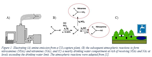
Along with the widely employed amine-technology comes the risk of forming carcinogenic and potentially carcinogenic nitrosamines (NSAs) and nitramines (NAs), respectively (Figure 1). These will form in the atmosphere from amines that inevitably escape the capture plant [1, 5]. Both compound groups are highly water-soluble, and concern is related to these ending up in nearby drinking water sources (e.g., groundwaters, lakes, etc.). In Norway, a drinking water safety limit has been set at 4 ng L-1 for the sum of NSAs and NAs [6]. Comparably low safety limits exist in other countries, but only for selected NSAs (e.g., action level of 3 ng L-1 in California; monitoring requirement at 1 ng L-1 in England and Wales) [7, 8].
Recent measurements at pilot CO2 capture plants indicate amine emissions in the ppb to ppm range, and with the levels being expectedly higher at a full-scale capture plant. The amount of emitted amines that will be converted to NSAs and NAs is governed by local air chemistry as well as the type of amines used at the capture plant. The atmospheric reaction is fast and proceeds with initial attack on the amine by an atmospheric oxidant (e.g., OH*) to form an amine radical. Subsequently, the amine radical reacts with a nitrogen oxide (NOx) to form either a NSA or a NA [1, 5, 9]. Primary amines such as 2-amino-2-methyl-1-propanol (AMP) and monoethanolamine (MEA) will form stable NAs while the corresponding NSAs will be unstable. Secondary amines (e.g. piperazine) can form both stable NSAs and NAs. Tertiary amines (e.g. methyldiethanolamine) will be degraded to secondary amines which can then react to form stable NSAs and NAs [10].
To assess whether the location of a sourced drinking water compartment is at risk of receiving NSAs and NAs above the safety limit, factors such as local weather and topography as well as degradation processes are decisive. For example, the dominating wind direction and speed will influence where the NSAs and NAs are likely to be deposited. Once on ground, they will follow the hydrological flow regime with overland flow, soil-pore and groundwater flow, from rivers into lakes. During daylight, NSAs are rapidly photodegraded on timescales ranging from minutes to hours [11-13]. By contrast, no efficient degradation pathway has been identified for NAs. Thus, there is a risk of NAs accumulating in a water compartment over time. One contended degradation pathway that has not been thoroughly investigated is biodegradation. Only one study has been conducted, reporting slow or no biodegradation for NAs in lake water [14].
In Norway, amine-based CO2 capture activities must comply to the drinking water safety limit [6]. This is carried out by limiting the amount of amines emitted with the cleaned flue gas. Amine emission permits are set in a site- specific manner, based on the drinking water limit, and by back-calculating from a nearby drinking water compartment. The estimates are conservative and based on rudimentary atmospheric modelling [15]. One reason for this simplified approach is the current lack of analytical methods capable of determining NAs in water at the required low level of the drinking water limit [16]. Instead, concentrations of amines in the emitted flue gas can be determined at low levels and with high certainty [17, 18]. However, there are shortcomings to the method currently used for estimating amine emission permits. This covers fundamental approximations used to describe the plume, the lack of validation through measurements, and the lack of incorporating the catchment processes. Moreover, to adhere to the precursory principle, worst case conditions are adopted at nearly all stages of the calculations where high uncertainty is related to the parameter value. Thus, this may lead to unrealistic and strict amine emission permits, thereby exerting unwarranted constraints to the technology.
The Technology Centre Mongstad (TCM) in Norway is the world’s most advanced and flexible test arena for CO2 capture technologies and is visited by private companies from all over the world. The site is near to several lakes that serve as drinking water sources for the local population [15]. This has resulted in low amine emission permits which currently restrict operations at TCM. To enable tests of the full range of amine solvents and flue gas compositions relevant for the industry, special concessions must be sought for from the environmental regulators. Considering that the size of the TCM facility constitutes only a fraction of a full-scale CO2 capture plant, it is likely that full-scale plants will require extensive and costly amine emission mitigation measures to remain within the permit. And given that the permit is calculated using the current method and knowledge base. Examples of amine emission mitigation options cover a reduced CO2 capture rate, additional rinsing of the flue gas or reheat of the flue gas prior to emission. These are costly options that will lead to a net reduction in the CO2 removal rate.
To ensure safe and cost-efficient implementation of amine-based CO2 capture technology, there is an urgent need to improve the method used to calculate the amine emission permits. New calculation methods should be based on new scientific evidence and an improved knowledge base safeguarding drinking water quality while at the same time avoiding unnecessary strict regulations of the capture process. We propose that this can be achieved through
1) an improved atmospheric model predicting the formation and transport of NSAs and NAs,
2) validating the new atmospheric model by in-plume and laboratory measurements,
3) coupling the atmospheric model to an existing catchment model, and
4) accounting for NAs potential biodegradation along flow paths within the catchment.
Herein we describe ongoing activities targeted to achieve these ambitious objectives. This is within the scope of the ongoing project, “Future drinking water levels of nitrosamines and nitramines near a CO2 capture plant (FuNitr)”.
2. Improved atmospheric model
In most instances, NSAs and NAs will form as products from reactions between constituents in the flue gas (amines) and in the background atmosphere (oxidants and NOx). Atmospheric oxidants are naturally present at background levels or stem from certain types of industrial activities in the vicinity. Sources of NOx are dominantly anthropogenic such as vehicular traffic or as constituents of the flue gas itself. For the chemical reactions to occur, the amine must encounter the oxidant and subsequently the NOx. Thus, to simulate NSA and NA formation and deposition rates, a realistic description of the plume dispersion and mixing is a prerequisite. The dilution of the emitted plume and the consequent contact between emitted and pre-existing chemical compounds occurs at a rate controlled by atmospheric turbulent mixing. To be able to integrate this into a model both the turbulent dispersion and the amine atmospheric chemistry must be adequately described.
This can be archived by using a special case mixing plume in grid Lagrangian Stochastic (LS) model which can be combined with an atmospheric chemistry transport model adapted for lower computational costs (EPISODE). The latter will cover the complex non-linear gas phase chemistry of amines. Characteristic for a standard LS model is its ability to simulate plume movement using a large number of notional particles [19, 20]. An LS model with mixing implies that the emitted particles are simulated together with particles representing the atmospheric background. The resolution is defined by the number of particles, which can be set high to realistically simulate the extreme dynamics of the plume. The mixing module describes encounters between the reactant compounds [21, 22], and simulates the decay of turbulent concentration fluctuations at the rate driven by the turbulent flow [21-23]. The explicit modelling of turbulent mixing implies that no approximations of the averaging operators are needed when solving a non-linear kinetic equation (chemistry appears in closed form) [22], which is typically required in other commonly used atmospheric chemistry transport models.
3. Validating atmospheric measurements
Two different sets of validation measurements will contribute to increase the accuracy of the atmospheric simulations. The first is to validate the NSA and NA atmospheric formation rates under realistic conditions. These have previously been experimentally determined, but only under ideal conditions in a large outdoor simulation chamber [24]. Second, there is a need to validate the output of the atmospheric model which has not previously been conducted in this context.
3.1 Atmospheric NSA and NA formation rates
At TCM there is a worldwide unique small laboratory placed on top of the absorption tower, where the treated flue gas is released to the atmosphere. This allows for the study of amine processing under near-real conditions. The atmospheric chemical transformations can be studied by leading the amine-treated flue gas into a small atmospheric simulation chamber.
3.2 In-situ plume measurements
In-situ plume measurements will be carried out by equipping a helicopter with state-of-the-art instrumentation capable of determining amines, NSAs, and NAs, in addition to NOx (NO and NO2), solar radiation (including NO2 photolysis frequency), etc. Such instrumentation must be ultra-sensitive and fast (1 Hz) to capture the low atmospheric levels from a rapidly moving helicopter. Aerial measurements are required since it is not possible to properly measure a wandering plume using fixed position measurements [25, 26].
4. Connecting the atmospheric model to a catchment model
To realistically simulate future levels of NSA and NA in a water compartment, catchment processes must be considered alongside the atmospheric processes. Moreover, the inclusion of the catchment processes will allow for assessing the possibility of NSAs and NAs to accumulate in the water with time. This can be done by running the atmospheric model in combination with a catchment model.
The importance of including the catchment module has already been demonstrated both for a lake- and a groundwater drinking water reservoir, as presented below. This was done using the INCA-Contaminant model [27] which is a high-resolution and dynamic catchment model, building on the hydrology model PERSiST [28]. Following deposition of NSAs and NAs on the ground, the catchment model simulates NA and NSA transportation to the lake or groundwater basin with soil- and groundwater runoff. The model is fed with site-specific numeric information, including catchment characteristics and climatic conditions to establish a site-specific scenario. More information about the model framework can be found here: nivanorge.github.io
4.1 Case study: lake
In the situation of a lake, NSAs and NAs will be supplied to the lake both directly from atmospheric deposition and with runoff draining the entire catchment. The study site was a lake located “downwind” from a planned full- scale CO2 capture plant [2]. A nearby high trafficked road contributed with excess NOx. The catchment model was fed with NSA and NA deposition rates and concentrations computed using a rudimentary atmospheric model. Continuous CO2 capture for ~20 y was assumed.
Results showed distinct long-term seasonal patterns in the lake water levels of NSAs and NAs (Figure 2) which reflected different response to key processes between the two compound groups. While the levels of NSAs were found to be relatively low and stable, the levels of NAs increased for approximately seven years before steady-state conditions were reached. The striking difference between the two compound groups was primarily the consequence of efficient photodegradation of the NSAs. Peak NSA levels occurred in winter when the lake was covered by ice and thereby protected from sunlight degradation. At this site, the sum of NSAs and NAs was likely to remain below the
drinking water limit of 4 ng L-1, but only when “reheat” was applied at the capture plant. By using reheat, the flue gas will literally be reheated to gain higher elevation and thereby enhanced atmospheric dispersion.
A model uncertainty analysis was run to reveal that the most uncertain and influential process is the biodegradation of the NAs. Since the NAs are not photodegraded, biodegradation is a potential important degradation pathway that can take place in soils, water, and sediment. To improve the accuracy of the simulation, future work should implement the atmospheric model described above as well as improving the knowledge on the potential for biodegradation of the NAs.
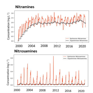
Figure 2: Modelled time series (2000-2020) of nitramines (NA, top) and nitrosamines (NSA, bottom) concentrations in the top (epilimnion) and bottom (hypolimnion) layers of the lake. Adapted from [2].
4.2 Case study: groundwater
A groundwater basin will receive NSAs and NAs mainly from soil-water percolation. One major concern is the lack of photodegradation taking place once the NSAs have reached the basin. This may lead to elevated levels of NSAs. At a case study site, two different groundwater basins were in close vicinity to a planned full-scale CO2 capture plant [29]. The two basins differed with respect to water residence time, water volume, and depth of the aquifers.
At both two sites, the levels of NSAs and NAs increased for an extended period (10-25 y) until steady state conditions were reached. The duration of this initial phase was dependent on the water residence time. A shorter water residence time translated into a faster increase in the NSA and NA levels. Since photodegradation was not in effect in the groundwater basin, the role of biodegradation was even more important, and also for the NSAs. Again, the process of biodegradation was found to have a large impact on the resulting NSA and NA concentrations, and at the same time being associated with a relatively high uncertainty.
To illustrate the importance of biodegradation, Figure 3 shows the continued increase in NSA and NA levels in the groundwater basin when no biodegradation is allowed to take place. For this site, the drinking water limit was exceeded after 25 years. It is important to note that this scenario without any biodegradation is a very unlikely scenario.
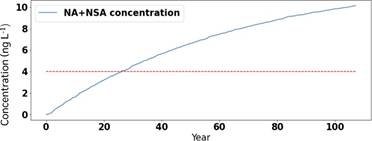
Figure 3: Modelled concentrations for the sum of NSAs and NAs (blue line) in a groundwater basin over time with no biodegradation in the groundwater. The red dotted line indicates the Norwegian recommended drinking water safety limit.
5. Experimental work to improve the catchment model (NA biodegradability)
Biodegradation has been identified as a key process associated with high uncertainty [2, 29]. Relevant NAs have simple molecular structures with a high N:C ratio, which are conceptually positively linked to biodegradability [30]. Moreover, a low microbial toxicity has been demonstrated [14, 31]. Two different experimental approaches have been suggested to improve the knowledge base and to produce new biodegradation rates to be used in the model.
The first approach is to further explore the biodegradability of the NAs in the water phase. The previous study on biodegradation of NAs in lake waters[14] showed that the potential for biodegradation varied with chemical structure of the nitramines, from no degradation to a slow degradation. And that for those that degraded, the slow biodegradation was mostly a result from a long lag-phase, which is the time needed by the microbes to adapt to a new type of substrate. Building on this, further assessments should test the effect of
1) exposing the microbial community to NAs over time,
2) mixing the different nitramines in the same test set-up,
3) varying the nutrient composition, and
4) varying the source and composition of the microbial inoculum.
The second approach is to assess the possibility for the NAs to be biodegraded in soil. In the catchment situation, soils typically constitute a large fraction of the area that the NAs must pass through to reach groundwater or a lake. In soils, there is typically a higher species diversity and number of microbes than in lake water. To our knowledge, this has not previously been investigated.
6. Open access modelling tool
To make the advanced atmospheric-catchment model available to the stakeholders, a user-friendly web-interface can be developed. Such a tool can aid authorities and the industry with the regulation and reduction measures, respectively, of the amine emissions. The website will visualise, in a simplified manner, the complex estimates and considerations taken by the model. The user can easily adjust settings on a selected range of input variables, such as CO2 capture operational conditions, to see the instant effect on NSA and NA levels in a nearby water compartment. All proprietary information will be anonymized and different chemical scenarios (e.g., amines with different atmospheric lifetimes and NSA/NA yields) will be presented.
7. Conclusions
Given the current political push to implement CO2 capture, there is an urgent need to create the tools and knowledge needed to support safe and knowledge-based implementation without compromising on the cost-efficiency. For the amine-technology, we here present a roadmap based on improving the simulations from measured amine emissions to future levels of NSAs and NAs at a nearby drinking water compartment. This will be done by adopting a fundamental new atmospheric model that will be validated using in-situ measurements. Subsequently, the atmospheric model will be combined with a catchment model to be able to simulate the entire picture from plant amine emissions
to water NSA and NA levels, and to also assess the potential for accumulation of NSAs and NAs with time. To further improve the accuracy of the model, the biodegradability of the NAs will be experimentally determined under realistic lake and soil conditions. Finally, to make the advanced developments available to the stakeholders, a user-friendly web-interface will be developed. With the tool, the instant effect from e.g. amine emission mitigation options can be visualized.
Acknowledgements
The work here presented is part of the ongoing project, Future drinking water levels of nitrosamines and nitramines near a CO2 capture plant (FuNitr) which has been funded by the Research Council of Norway (#336357), under the CLIMIT-programme.
References
[1] C.J. Nielsen, H. Herrmann, C. Weller, Atmospheric chemistry and environmental impact of the use of amines in carbon capture and storage (CCS), Chemical Society Reviews, 41 (2012) 6684-6704. http://dx.doi.org/10.1039/C2CS35059A.
[2] M.D. Norling, F. Clayer, C.B. Gundersen, Levels of nitramines and nitrosamines in lake drinking water close to a CO2 capture plant: A modelling perspective, Environmental Research, 212 (2022) 113581. https://doi.org/10.1016/j.envres.2022.113581.
[3] Global CCS Institute, Global status of CCS 2023. Scaling up through 2030, 2023, https://status23.globalccsinstitute.com/.
[4] European commission, Towards an ambitious industrial carbon management for the EU, European Commission, Directorate- General for Energy, 2024, https://eur-lex.europa.eu/legal-content/EN/TXT/?uri=COM:2024:62:FIN.
[5] J.N. Pitts, Jr., D. Grosjean, K. Van Cauwenberghe, J.P. Schmid, D.R. Fitz, Photooxidation of aliphatic amines under simulated atmospheric conditions: formation of nitrosamines, nitramines, amides, and photochemical oxidant, Environmental Science & Technology, 12 (1978) 946-953. https://doi.org/10.1021/es60144a009.
[6] C. Svendsen, M. Låg, B. Lindeman, M. Andreassen, B. Granum, New knowledge on health effects of amines and their derivatives associated with CO2 capture, Norwegian Institute of Public Health (NIPH), Oslo, Norway, 2024, https://www.miljodirektoratet.no/publikasjoner/2024/januar-2024/new-knowledge-on-health-effects-co2-capture/.
[7] J. Nawrocki, P. Andrzejewski, Nitrosamines and water, J Hazard Mater, 189 (2011) 1-18. https://doi.10.1016/j.jhazmat.2011.02.005.
[8] California Water Boards, Nitrosamines, State Water Resources Control Board, Division of Drinking Water, Regulatory Development Unit, Sacramento, California, USA, 2024, https://www.waterboards.ca.gov/drinking_water/certlic/drinkingwater/NDMA.html.
[9] N.R. Choi, S. Park, S. Ju, Y.B. Lim, J.Y. Lee, E. Kim, S. Kim, H.J. Shin, Y.P. Kim, Contribution of liquid water content enhancing aqueous phase reaction forming ambient particulate nitrosamines, Environmental Pollution, 303 (2022) 119142. https://doi.org/10.1016/j.envpol.2022.119142.
[10] N. Dai, A.D. Shah, L. Hu, M.J. Plewa, B. McKague, W.A. Mitch, Measurement of nitrosamine and nitramine formation from NOx reactions with amines during amine-based carbon dioxide capture for postcombustion carbon sequestration, Environmental Science & Technology, 46 (2012) 9793-9801. https://doi.org/10.1021/es301867b.
[11] A. Afzal, J. Kang, B.-M. Choi, H.-J. Lim, Degradation and fate of N-nitrosamines in water by UV photolysis, International Journal of Greenhouse Gas Control, 52 (2016) 44-51. https://doi.org/10.1016/j.ijggc.2016.06.009.
[12] M.H. Plumlee, M. Reinhard, Photochemical attenuation of N-nitrosodimethylamine (NDMA) and other nitrosamines in surface water, Environmental Science & Technology, 41 (2007) 6170-6176. 10.1021/es070818l, https://doi.org/10.1021/es070818l.
[13] L. Sørensen, K. Zahlsen, A. Hyldbakk, E.F.d. Silva, A.M. Booth, Photodegradation in natural waters of nitrosamines and nitramines derived from CO2 capture plant operation, International Journal of Greenhouse Gas Control, 32 (2015) 106-114. https://doi.org/10.1016/j.ijggc.2014.11.004.
[14] O.G. Brakstad, L. Sørensen, K. Zahlsen, K. Bonaunet, A. Hyldbakk, A.M. Booth, Biotransformation in water and soil of nitrosamines and nitramines potentially generated from amine-based CO2 capture technology, International Journal of Greenhouse Gas Control, 70 (2018) 157-163. https://doi.org/10.1016/j.ijggc.2018.01.021.
[15] M. Karl, N. Castell, D. Simpson, S. Solberg, J. Starrfelt, T. Svendby, S.E. Walker, R.F. Wright, Uncertainties in assessing the environmental impact of amine emissions from a CO2 capture plant, Atmospheric Chemistry and Physics, 14 (2014) 8533- 8557. https://doi.10.5194/acp-14-8533-2014, https://doi.10.5194/acp-14-8533-2014.
[16] S. Lindahl, C.B. Gundersen, E. Lundanes, A review of available analytical technologies for qualitative and quantitative determination of nitramines, Environmental Science: Processes & Impacts, 16 (2014) 1825-1840. https://doi.10.1039/c4em00095a.
[17] W. Tan, L. Zhu, T. Mikoviny, C.J. Nielsen, Y. Tang, A. Wisthaler, P. Eichler, M. Müller, B. D’Anna, N.J. Farren, J.F. Hamilton, J.B.C. Pettersson, M. Hallquist, S. Antonsen, Y. Stenstrøm, Atmospheric chemistry of 2-amino-2-methyl-1-propanol: A theoretical and experimental study of the OH-initiated degradation under simulated atmospheric conditions, The Journal of Physical Chemistry A, 125 (2021) 7502-7519. https://doi.org/10.1021/acs.jpca.1c04898.
[18] W. Tan, L. Zhu, T. Mikoviny, C.J. Nielsen, A. Wisthaler, B. D’Anna, S. Antonsen, Y. Stenstrøm, N.J. Farren, J.F. Hamilton, G.A. Boustead, A.D. Brennan, T. Ingham, D.E. Heard, Experimental and theoretical study of the OH-initiated degradation of piperazine under simulated atmospheric conditions, The Journal of Physical Chemistry A, 125 (2021) 411-422. https://doi.org/10.1021/acs.jpca.0c10223, https://doi.org/10.1021/acs.jpca.0c10223.
[19] D. Thomson, J. Wilson, History of Lagrangian stochastic models for turbulent dispersion, 2012, pp. 19-36 https://doi.org.10.1029/2012GM001238.
[20] M. Cassiani, A. Stohl, J. Brioude, Lagrangian stochastic modelling of dispersion in the convective boundary layer with skewed turbulence conditions and a vertical density gradient: Formulation and implementation in the FLEXPART model, Boundary-Layer Meteorology, 154 (2015) 367-390. https://doi.org/10.1007/s10546-014-9976-5.
[21] M. Cassiani, P. Franzese, U. Giostra, A PDF micromixing model of dispersion for atmospheric flow. Part 1: development of the model, application to homogeneous turbulence and to neutral boundary layer, Atmospheric Environment, 39 (2005) 1457- 1469. https://10.1016/j.atmoshere.2004.11.020.
[22] R. Fox, Computational Models for Turbulent Reacting Flow, 2003.
[23] M. Cassiani, M.B. Bertagni, M. Marro, P. Salizzoni, Concentration fluctuations from localized atmospheric releases, Boundary-Layer Meteorology, 177 (2020) 461-510. https://doi.org/10.1007/s10546-020-00547-4.
[24] W. Tan, L. Zhu, T. Mikoviny, C.J. Nielsen, A. Wisthaler, P. Eichler, M. Müller, B. D’Anna, N.J. Farren, J.F. Hamilton, J.B.C. Pettersson, M. Hallquist, S. Antonsen, Y. Stenstrøm, Theoretical and experimental study on the reaction of tert-butylamine with OH radicals in the atmosphere, The Journal of Physical Chemistry A, 122 (2018) 4470-4480. https://doi.org/10.1021/acs.jpca.8b01862.
[25] M. Luria, R.J. Valente, R.L. Tanner, N.V. Gillani, R.E. Imhoff, S. F. Mueller, K.J. Olszyna, J.F. Meagher, The evolution of photochemical smog in a power plant plume, Atmospheric Environment, 33 (1999) 3023-3036. https://doi.org/10.1016/S1352- 2310(99)00072-2.
[26] M. Luria, R.L. Tanner, R.E. Imhoff, R.J. Valente, E.M. Bailey, S.F. Mueller, Influence of natural hydrocarbons on ozone formation in an isolated power plant plume, Journal of Geophysical Research: Atmospheres, 105 (2000) 9177-9188. https://doi.org/10.1029/1999JD901018.
[27] L. Nizzetto, D. Butterfield, M. Futter, Y. Lin, I. Allan, T. Larssen, Assessment of contaminant fate in catchments using a novel integrated hydrobiogeochemical-multimedia fate model, Science of the Total Environment, 544 (2016) 553-563. https://doi.10.1016/j.scitotenv.2015.11.087.
[28] M.N. Futter, M.A. Erlandsson, D. Butterfield, P.G. Whitehead, S.K. Oni, A.J. Wade, PERSiST: a flexible rainfall-runoff modelling toolkit for use with the INCA family of models, Hydrology and Earth System Sciences, 18 (2014) 855-873. https://doi.10.5194/hess-18-855-2014.
[29] C.B. Gundersen, M.D. Norling, A.S. Gragne, Modelling future levels of nitrosamines and nitramines in a groundwater compartment close to a CO2 capture facility, Norwegian institute for water research (NIVA), 2024, https://niva.brage.unit.no/niva-xmlui/handle/11250/3160694.
[30] K. Kalbitz, J. Schmerwitz, D. Schwesig, E. Matzner, Biodegradation of soil-derived dissolved organic matter as related to its properties, Geoderma, 113 (2003) 273-291. https://doi.org/10.1016/S0016-7061(02)00365-8.
[31] C.B. Gundersen, T. Andersen, S. Lindahl, D. Linke, R.D. Vogt, Bacterial response from exposure to selected aliphatic nitramines, Energy Procedia, 63 (2014) 791-800. https://doi.org/10.1016/j.egypro.2014.11.089, https://www.sciencedirect.com/science/article/pii/S1876610214019043.
CESAR1 Solvent Degradation in Pilot and Laboratory Scale (2024)
Vanja Buvika*, Andreas Grimstvedta, Kai Vernstada, Merete Wiiga, Hanna K. Knuutilab, Muhammad Zeeshanc, Sundus Akhterc, Karen K. Høisæterc, Fred Rugenyic, Matthew Campbellc
*Corresponding author. Email address: vanja.buvik@sintef.no
aSINTEF Industry, NO-7465 Trondheim, Norway
bDepartment of Chemical Engineering, Norwegian University of Science and Technology (NTNU), N-7497- Trondheim, Norway
cTechnology Centre Mongstad, NO-5954 Mongstad, Norway
Abstract
A CESAR1 solvent sample which had been subjected to a series of test campaigns with industrial flue gases was analysed for identified degradation compounds with newly developed analytical techniques. Before analysing the pilot sample, the degradation compounds of CESAR1 were identified in samples from laboratory scale oxidative and thermal degradation stress tests with aqueous 2-amino-2-methyl-propanol (AMP), piperazine (PZ) and the CESAR1 blend. Three new major degradation compounds, which have previously not been identified, were found among the ten most abundant degradation species. A total of 35 degradation compounds were found in the solvent sample, whereof 12 have not been previously identified neither in CESAR1 nor during degradation of AMP or PZ alone. By comparing the quantified solvent amines and degradation compounds with the total concentration of nitrogen in the sample, it was found that all major nitrogen containing degradation compounds are accounted for, and that the nitrogen containing species in the solvent have been identified and quantified within the analytical uncertainty. This contributes to closing one of the major knowledge gaps associated with CO2 capture operations with the CESAR1 solvent, which is a target of the Horizon Europe project AURORA.
Keywords: AMP, piperazine, stability, oxidative and thermal degradation
1. Introduction
The non-proprietary CESAR1 amine blend has been widely studied for use as a solvent for post-combustion CO2 capture (Campbell et al., 2022; Knudsen et al., 2011; Mangalapally and Hasse, 2011; Moser et al., 2023; Rabensteiner et al., 2016). Despite of its relative popularity in the solvent market, there are still many knowledge gaps connected to the stability of CESAR1 (Morlando et al., 2024). The mixture of 2-amino-2-methyl propanol (AMP, CAS 124-68-5) and piperazine (PZ, CAS 110-85-0) is known to be much more stable than ethanolamine (MEA, CAS 141-43-5), both under oxidising conditions, thermal stress, and at the cyclic conditions in the CO2 capture plant.
Even though the stability of CESAR1 is higher compared to other solvents, the degradation phenomena still need to be fully understood before the solvent can be safely implemented for large or full-scale CO2 capture from industrial sources. Amine solvents degrade due to reactions between the amine and reactive species present in the flue gas (such as O2, SOX and NOX.), high temperatures and presence of catalytic amounts of dissolved metals (Buvik et al., 2021; Dumée et al., 2012; Flø et al., 2017; Vega et al., 2020). The degradation can lead to reduced process efficiency, high solvent replacement and reclaiming costs, as well as corrosion or fouling of the construction materials. If the degradation compounds that form are more volatile than the solvent amine(s), it can also lead to increased emissions into the atmosphere where they can impact the environment. Understanding solvent degradation is therefore important from both environmental, economic, and safety perspectives.
All amines produce some generic degradation products, like carboxylates (i.e., formate, acetate, etc.), aldehydes (formaldehyde, acetaldehyde), and ammonia (Vevelstad et al., 2022). Additionally, they will produce solvent specific compounds, which will depend on the chemical structure of the amine in use. For CESAR1, although many potential degradation products have been suggested in the literature, especially through studies on AMP and PZ (Eide-Haugmo et al., 2011; Freeman et al., 2010; Freeman and Rochelle, 2012; Lepaumier et al., 2009; Wang and Jens, 2014, 2012), only a limited number of degradation compounds were previously known. A thorough review of identified and suggested degradation compounds of AMP, PZ and their blends can be found in Morlando et al. (2024).
Despite of solvent degradation being low compared to other solvents, degradation phenomena need to be fully understood before a solvent can be safely implemented for large or full-scale CO2 capture from industrial sources, to fully comprehend potential environmental and operational impacts, and ensure safety for operators and neighbouring community. Therefore, this study aims to fully characterise the degraded CESAR1 solvent, to identify all the remaining compounds. To achieve this, analysis of the total (molar) concentration of nitrogen in the solvent is compared to the total (molar) concentration of nitrogen in known compounds, meaning the sum of nitrogen in AMP, PZ, known contaminants and degradation compounds. The literature has previously stated that about 50% of the nitrogen containing degradation compounds in AMP and PZ remain unidentified (Wang, 2013; Wang and Jens, 2014).
2. Materials and methods
2.1 Pilot samples
In the period from late 2019 to the end of 2020, Technology Centre Mongstad (TCM) ran multiple test campaigns to study the behaviour of the CESAR1 solvent at their post-combustion CO2 capture plant. These included the ALIGN CCUS CESAR1 campaign and two CESAR1 campaigns by the TCM owners (Benquet et al., 2021; Bui et al., 2022; Campbell et al., 2022; Drageset et al., 2022; Hume et al., 2021; Languille et al., 2021a, 2021b). During these campaigns that were conducted successively at TCM, the solvent was subjected to both combined heat and power (CHP) flue gas and residue fluid catalytic cracking (RFCC) flue gas. In addition, two rounds of thermal reclaiming were conducted, and make-up solvent was added when needed. Altogether, the solvent sample studied in this work was in use in the TCM plant for about 13 months in total, and the analysed sample was taken after the plant was drained.
2.2 Oxidative and thermal degradation experiments
To get a more detailed understanding of the degradation seen at the pilot scale, some laboratory experiments were performed. In those experiments, AMP and PZ with purity of 99% was used to prepare the aqueous solutions of 3.0 mol/kg AMP, 1.5 mol/kg PZ, and the CESAR1 blend (3.0 mol/kg AMP + 1.5 mol/kg PZ). The solutions were gravimetrically preloaded with pure CO2 to the desired loading and analysed for amine and CO2 content to ensure correct loading before use in the experiments.
Oxidative degradation of the single amines and CESAR1 blend was performed according to Vevelstad et al. (2016) in a water bath heated double-jacketed glass reactor at 60 °C with 50 L/min of gas bubbled through the solution and circulated back to the solution. The solvent, pre-loaded with CO2 to contain 0.4 mol CO22 per mol amine functionality was used in the experiments. A catalytic amount of iron sulphate heptahydrate (FeSO4‧7H2O, 0.5 mmol/L) was added to the solvent. A small amount of gas (77% N2, 21% O2, 2% CO2) was continuously added to the reactor to ensure constant O2 concentration. A bleed leaving the reactor was taken through two double-jacketed condensers before exiting through two impinger bottles containing 0.1 M H2SO4 (aq.). Liquid samples were taken regularly, and a 2,4-dinitrophenylhydrazine (DNPH) cartridge was attached between the second condenser and the first impinger bottle for the last 4 days of the experiment.
Testing of the thermal stability of AMP, PZ and CESAR1 was performed in closed SS316L cylinders according to Lepaumier et al. (2011) over a period of 28 days, and some cylinders were withdrawn regularly for analyses. The temperature of 135 °C was used in all experiments and the solutions were loaded up to 0.4 mol CO2 per mol amine functionality.
2.3 Analytical methods
SINTEF evaluated nearly 100 potential degradation compounds. The basis for the evaluation was compounds proposed for AMP, PZ and their blends in the existing literature (Morlando et al., 2024) and analogous degradation mechanisms known for amines other than the CESAR1 components (Vevelstad et al., 2022). Compounds to analyse were selected based on their likelihood of formation and the possibility of obtaining analytical standards for method development. SINTEF already had analytical methods for many compounds. For others, SINTEF purchased analytical standards and developed LCMS quantification methods. The main goal was to be able to close the nitrogen balance of degraded CESAR1 samples. The LC-MS/MS methods used in this work are based on the same principles as those described in Vevelstad et al. (2023). An overview of compounds analysed using LC-MS/MS in the degraded solvent samples is given in Table 1.
Table 1: Compounds analysed in the degraded solvent samples.
| Abbrev. | Name | CAS-number |
| AAc | Acetic acid | 64-19-7 |
| – | Acetaldehyde | 75-07-0 |
| – | Acetone | 67-64-1 |
| AAEA | 2-amino-N-(2-aminoethyl)-acetamide | 84354-31-4 |
| AEAAC | N-(2-aminoethyl)-glycine | 24123-14-6 |
| AEAEPZ | 1-[2-(1-piperazinyl) ethyl]-1,2-ethanediamine | 24028-46-4 |
| AEAEPZ urea | 1-[2-(1-piperazinyl) ethyl]-2-imidazolidinone | 104087-61-8 |
| AEHA | N-(2-aminoethyl)-2-hydroxy- acetamide | 83019-76-5 |
| AEI | 1-(2-aminoethyl)-2-imidazolidone | 6281-42-1 |
| AIBA | 2-Aminoisobutyric acid | 62-57-7 |
| AMPAMP | 2-[(2-amino-2-methylpropyl)amino]-2-methyl-1-propanol | 72622-74-3 |
| AMP-NO2 | 2-methyl-2-(nitroamino)-1-propanol | 1239666-60-4 |
| AMPPZ | 2-amino-2-methyl-1-(1-piperazinyl)-1-propanone | 479065-33-3 |
| AMP urea | N,N‘-bis(2-hydroxy-1,1-dimethylethyl)-urea | 162748-76-7 |
| DAEP | 1,4-piperazinediethanamine | 6531-38-0 |
| DEA | Diethylamine | 109-89-7 |
| DFP | 1,4-piperazinedicarboxaldehyde | 4164-39-0 |
| DMA | dimethylamine | 124-40-3 |
| DMHTBI | 4,4-dimethyl-1-hydroxytertbutyl-2-imidazolidinone | 2761991-15-3 |
| DMOZD | 4,4-dimethyl-2-oxazolidinone | 26654-39-7 |
| DMP | 1,4-dimethylpiperazine | 160-58-1 |
| DM-PZEA | α,α-dimethyl-1-piperazineethanamine | 1259927-55-3 |
| DNPZ | N,N’-dinitrosopiperazine | 140-79-4 |
| DPA | Dipropylamine | 142-84-7 |
| EA | Ethylamine | 75-04-7 |
| EDA | Ethylenediamine | 107-15-3 |
| EMA | Ethylmethylamine | 624-78-2 |
| EPZ | 1-ethylpiperazine | 5308-25-8 |
| F-AMP | N-(2-hydroxy-1,1-dimethylethyl)formamide | 682-85-9 |
| FAc | Formic acid | 64-18-6 |
| – | Formaldehyde | 50-00-0 |
| FPZ | 1-piperazinecarboxaldehyde | 7755-92-2 |
| GAc | Glycolic acid | 79-14-1 |
| HEP | 1-piperazineethanol | 103-76-4 |
| HMeGly | N-(2-hydroxy-1,1-dimethylethyl)-Glycine | 1154902-47-2 |
| HPAc | 3-hydroxypropanoic acid | 503-66-2 |
| HTBI | 1-(1-Hydroxy-2-methylpropan-2-yl)imidazolidin-2-one | 1566510-82-4 |
| iBAc | Isobutyric acid | 79-31-2 |
| LAc | Lactic acid | 50-21-5 |
| MA | methylamine | 74-89-5 |
| MAMP | 2-methyl-2-(methylamino)-1-propanol | 27646-80-6 |
| MNPZ | N-nitrosopiperazine | 5632-47-3 |
| MPZ | 1-methylpiperazine | 109-01-3 |
| NMAMP | nitroso-N-methyl-2-amino-2-methylpropanol | 27646-81-7 |
| – | Ammonia | 7664-41-7 |
| OPZ | Piperazinone | 5625-67-2 |
| PA | Propylamine | 107-10-8 |
| PAc | Propionic acid | 79-09-4 |
| PEP | 1,1′-(1,2-ethanediyl)bis-piperazine | 19479-83-5 |
| PZ-NO2 | 1-nitropiperazine | 42499-41-2 |
| TMOX | 3,4,4-trimethyl-2-oxazolidinone | 15833-17-7 |
Analysis of total CO2 and total nitrogen (TN) concentration in the samples were performed on a Shimadzu TOC-LCPH with a TNM-L unit by SINTEF. Both systems were calibrated prior to use with NaHCO3 and ethanolamine, respectively.
3. Results and discussion
3.1 CESAR1 degradation compounds in the pilot sample
During the 2019 ALIGN CCUS campaign at TCM, samples were sent to SINTEF for quantification of selected and known degradation products at the time. These included 2,4-lutidine, 4,4-dimethyl-2-oxazolidione (DMOZD), N-methylpiperazine (MNPZ), 2-oxopiperazine (OPZ), formic acid (FAc), oxalic acid, glycolic acid (GAc), and propionic acid (PAc) (Benquet et al., 2021). Detailed results from this campaign have been described by Campbell et al. (2022). In this previous work, the total alkalinity was used to assess the state of the solvent. The observed results showed a deviation between the sum of known alkaline components in the sample and the measured total alkalinity, indicating the presence of unknown degradation products. Due to this, a sample from the end of the operation at TCM was characterized using the newly developed LC-MS/MS methods. The methods were used to analyse new degradation components in addition to the components analysed in the past. This work presents the results from the analysis of the sample from the end of operation of the 2019-2020 CESAR1 campaigns. It is important to note that, as the sample in question has been through multiple campaigns with different flue gas sources, including solvent make-up and thermal reclaiming, the ratio of the different degradation products is not necessarily representative of what would be found in a campaign solvent under normal operating conditions. It will, however, show which compounds can be expected to be seen under operation with CESAR1, and hence, contribute to closing knowledge gaps associated with CESAR1 degradation.
EDA, HMeGly, and TMOX were the most abundant degradation products found in the end of operations sample. Out of these three, HMeGly and TMOX have not previously been quantified in AMP, PZ, nor CESAR1 in the open literature. Figure 1 shows all the 33 components quantified in the sample from end of operation. Out of these 33 compounds, 11 AMP, PZ, or CESAR1-specific compounds have previously not been quantified. These include HMeGly, TMOX, DM-PZEA, AMPAMP, AMP-urea, AAEA, F-AMP, AIBA, AEHA, AEAEPZ, and PEP. Some additional generic degradation compounds that have also not been specifically reported to be found in CESAR1, namely HPAc, LAc, and EA were also found, as well as traces of two additional CESAR1-speficic compounds, AEAEPZ-urea and AMP-NO2. An additional 15 compounds not presented in the figure were below the quantitation limits of the methods used.
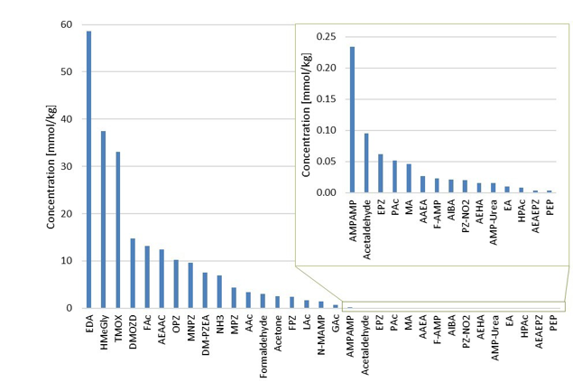
Figure 1: Concentrations of degradation compounds in CESAR1 solvent after ended operation at TCM.
When assessing the nitrogen balance, the total alkalinity only captures basic nitrogen-containing compounds which are partly neutralised by acidic components in the solvent (Waite et al., 2013). The total nitrogen provides a better assessment of the mass balance as it is not prone to the mentioned drawbacks. Total nitrogen (TN) analysis indiscriminately quantifies all nitrogen bound in any species (besides N2).
By adding up the nitrogen in all measured compounds and comparing this with the amount total nitrogen from the TN analysis, the contribution of the degradation products and the solvent amines to the nitrogen balance of the solvent can be assessed. Figure 2 shows that about 99% of the nitrogen in the solvent was accounted for. The solvent amines, AMP and PZ, account for 92% of the TN, while the quantified degradation products account for about 7% of the
nitrogen. Of these 7%, MAMP, which is a common contaminant in AMP found in the CESAR1 solvent before flue gas contact, accounted for around 1% of the TN. The degradation products which could be quantified by the previously available analytical methods, MNPZ, OPZ, and DMOZD, account for about 1%. Finally, the new degradation products presented in this work account for approximately 5% of the TN. The nitrogen balance closure from the newly identified and quantified degradation compounds underlines the value derived from the newly identified compounds and developed analytical methods in providing further insights into the behaviour of CESAR1. The analytical uncertainty of the TN analysis is ±10%, while that of each individual component is ±5%, making the 1% of nitrogen that is not accounted for insignificant. This does not mean that all degradation compounds of CESAR1 have been identified to date but indicates that all major nitrogen containing compounds are accounted for in this study.
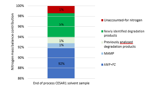
Figure 2: Summary of the nitrogen balance showing the contribution of AMP and PZ, previously quantified degradation products, newly identified degradation products and the unaccounted-for nitrogen. The unaccounted-for nitrogen could be due to uncertainties in the analytical methods used, unidentified degradation products or degradation compounds in concentrations below the limit of quantification of the measurement methods used or combinations thereof.
3.2 Comparison of the pilot samples to oxidative and thermal degraded AMP, PZ and CESAR1 blend
In the lab experiments, conditions that accelerate thermal or oxidative degradation are used. This allows relatively short experimental time and often leads to a degree of degradation that is not industrially acceptable, nor realistic. However, the advantage of these tests is that it is often easier to identify and analyse new degradation compounds as they are present in higher concentrations, and one can potentially find compounds that might otherwise only occur in quantifiable amounts after long-term operation. Furthermore, these laboratory scale tests allow for the identification of:
1) The conditions under which a compound forms (oxidative or thermal degradation), and
2) From which amines (PZ, AMP or both) they originate.
The main degradation compound (molar basis) of CESAR1 is EDA, which is a known oxidation product of PZ (Freeman et al., 2010). HMeGly is an amino acid that has not previously been identified or quantified in CESAR1, PZ or AMP. The laboratory experiments show that HMeGly is primarily formed during oxidative degradation of CESAR1, although some HMeGly is also formed in the thermal degradation experiments (maximum 5 mmol/kg). The concentration of HMeGly over time during oxidative degradation is shown in Figure 3a. The formation mechanism of HMeGly is likely to be analogous to that of N-(2-hydroxyethyl)-glycine (“HEGly”, CAS 5835−28-9) which is a major degradation compounds of MEA. Many reaction pathways for the formation of HEGly have been suggested (Vevelstad et al., 2016), without a clear consensus on which pathway is the most probable. HMeGly is likely to form through the same mechanism as HEGly in MEA, only with AMP as the reactant as opposed to MEA.
DM-PZEA is clearly a thermal degradation product that can only form in the blend of PZ and AMP, and not in each solvent separately. The concentration of DM-PZEA after 4 weeks of thermal degradation at 135°C in stainless steel cylinders is shown in Figure 3b. Oxidative degradation of CESAR1 gave a maximum DM-PZEA concentration of 4 mmol/kg after 6 weeks, while AMP and PZ alone never formed any DM-PZEA.
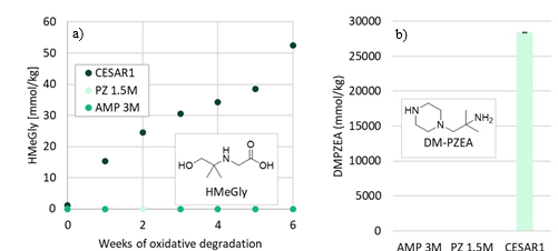
Figure 3: (a) Concentration of HMeGly during oxidative degradation experiments over time, and (b) concentration of DM-PZEA after thermal degradation at 135C in the presence of 0.4 mol CO2 per mol N.
DM-PZEA is suggested to form through a carbamate polymerisation type reaction, where the cyclic carbamate DMOZD reacts with PZ in a condensation reaction to form the “dimer” DM-PZEA, as shown in Figure 4. This degradation product was suggested by Li et al. (2013).
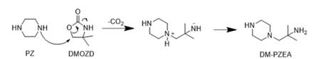
Figure 4: Suggested mechanism of formation of DM-PZEA.
TMOX is mainly a product of thermal MAMP degradation, and as MAMP is a common contaminant in technical AMP, TMOX can form during AMP and CESAR1 degradation as shown in Figure 5a. TMOX also forms to a lesser extent during oxidative AMP degradation, but is not present in significant amounts during oxidative degradation of the CESAR1 blend, as can be seen in Figure 5b. TMOX is hypothesised to form according to the mechanism described in Figure 6, by intramolecular condensation of the MAMP carbamate.
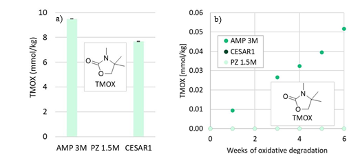
Figure 5: TMOX concentration (a) after thermal degradation at 135°C in the presence of 0.4 mol CO2 per mol N, and (b) during oxidative degradation.
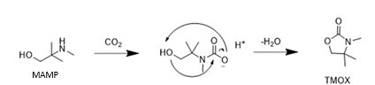
Figure 6: Suggested formation pathways of TMOX, analogously to that of DMOZD from AMP.
Another amino acid that is formed during CESAR1 degradation is AEAAC, which has been suggested to be a PZ degradation product in the literature (Freeman, 2011; Wang, 2013). This compound is likely formed through the same degradation mechanism as HMeGly and HEGly, where EDA is a likely reactant. The formation of AEAAC during laboratory scale oxidative degradation experiments is depicted in Figure 7a.
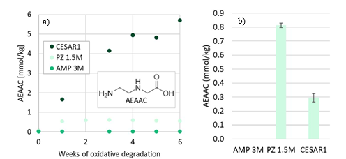
Figure 7: Concentration of AEAAC during (a) oxidative degradation experiments over time, and (b) after 4 weeks thermal degradation at 135°C with 0.4 mol CO2 per mol N.
Furthermore, DMOZD and AMPAMP are products of thermal AMP degradation. The oxidation products of PZ, OPZ and FPZ, form only in low concentrations during oxidative degradation of only PZ. Their formation rates, however, are greatly accelerated in the CESAR1 blend. MPZ and EPZ are thermal degradation products of PZ. Generally, all degradation reactions are accelerated in the CESAR1 blend compared to in the single amine 1.5M PZ or 3M AMP solvents. Despite the formation pathways in theory only requiring one of the species, the blend enhances formation in all cases except for the formation of AEAAC at thermally degrading conditions, shown in Figure 7b, in which case
more AEAAC was formed in PZ than in CESAR1. This can possibly be explained by the presence of competing reactants, i.e. AMP forming HMeGly with the same reactants as form AEAAC, and the HMeGly reaction having a lower activation energy.
4. Conclusions
In this work, 35 different degradation compounds were successfully identified and quantified in the degraded CESAR1 solvent that had been through a series of pilot tests at TCM. This was in addition to the solvent amines and a known contaminant in the solvent amine AMP (MAMP). 12 of these have never been identified nor quantified neither in PZ, AMP, or CESAR1. Additionally, 99% (±10%) of all nitrogen contained in a degraded CESAR1 sample that had been through testing at TCM have been successfully identified. With the previously available analytical methods, only 2% of all nitrogen in the sample, other than from solvent amines, could be identified. Now, with the new analytical methods in this work, 7% of all nitrogen could be identified. This is effectively more than tripling the known amount of nitrogen containing degradation products of CESAR1. 92% of the total nitrogen content of the sample originates from the solvent amines.
Nearly all degradation reactions take place more rapidly or to a larger extent in the CESAR1 blend than in the single amine solvents in the laboratory tests. Two amino acid degradation compounds, HMeGly and AEAAC, were quantified in large concentrations in the CESAR1 solvent. Their formation mechanism is not fully understood. Other degradation products, like TMOX, is likely formed analogously to DMOZD, which was already a known degradation product of AMP. The conditions under which the various degradation reactions take place were identified by comparing the analytical results from a sample of CESAR1 from pilot scale operation with real flue gas, to laboratory scale oxidative and thermal degradation experiments with the single amines and the CESAR1 solvent.
Acknowledgements
- The AURORA project, which has received funding from the European Union’s Horizon Europe research and innovation programme under grant agreement No. 101096521. https://aurora-heu.eu/
- This publication has been produced with support from the NCCS Research Centre, performed under the Norwegian research programme Centre for Environment-friendly Energy Research (FME). The
authors acknowledge the following partners for their contributions: Aker BP, Aker Carbon
Capture, Allton, Ansaldo Energia, Baker Hughes, CoorsTek Membrane Sciences, Elkem, Eramet, Equinor, Gassco, Hafslund Oslo Celsio, KROHNE, Larvik Shipping, Norcem Heidelberg Cement, Offshore
Norge, Quad Geometrics, Stratum Reservoir, TotalEnergies, Vår Energi, Wintershall DEA and the Research Council of Norway (257579/E20). https://nccs.no/
References
Benquet, C., Knarvik, A.B.N., Gjernes, E., Hvidsten, O.A., Romslo Kleppe, E., Akhter, S., 2021. First Process Results and Operational Experience with CESAR1 Solvent at TCM with High Capture Rates (ALIGN-CCUS Project). SSRN Journal. https://doi.org/10.2139/ssrn.3814712
Bui, M., Campbell, M., Knarvik, A., Tait, A., Baxter, X., Bowers, J., Mac Dowell, N., 2022. Evaluating Performance During Start-Up and Shut Down of the TCM CO2 Capture Facility.
Buvik, V., Høisæter, K.K., Vevelstad, S.J., Knuutila, H.K., 2021. A review of degradation and emissions in post- combustion CO2 capture pilot plants. International Journal of Greenhouse Gas Control 106, 103246. https://doi.org/10.1016/j.ijggc.2020.103246
Campbell, M., Akhter, S., Knarvik, A., Muhammad, Z., Wakaa, A., 2022. CESAR1 Solvent Degradation and Thermal Reclaiming Results from TCM Testing.
Drageset, A., Ullestad, Ø., Kleppe, E.R., McMaster, B., Aronson, M., Olsen, J.-A., 2022. Real-time monitoring of 2-amino-2-methylpropan-1-ol and piperazine emissions to air from TCM post combustion CO2 capture plant during treatment of RFCC flue gas. Available at SSRN 4276745.
Dumée, L., Scholes, C., Stevens, G., Kentish, S., 2012. Purification of aqueous amine solvents used in post combustion CO2 capture: A review. International Journal of Greenhouse Gas Control 10, 443–455. https://doi.org/10.1016/j.ijggc.2012.07.005
Eide-Haugmo, I., Lepaumier, H., da Silva, E.F., Einbu, A., Vernstad, K., Svendsen, H.F., 2011. A study of thermal degradation of different amines and their resulting degradation products, in: 1st Post Combustion Capture Conference. pp. 17–19.
Flø, N.E., Faramarzi, L., de Cazenove, T., Hvidsten, O.A., Morken, A.K., Hamborg, E.S., Vernstad, K., Watson, G., Pedersen, S., Cents, T., 2017. Results from MEA degradation and reclaiming processes at the CO2 Technology Centre Mongstad. Energy Procedia 114, 1307–1324.
Freeman, S.A., 2011. Thermal degradation and oxidation of aqueous piperazine for carbon dioxide capture. Freeman, S.A., Davis, J., Rochelle, G.T., 2010. Degradation of aqueous piperazine in carbon dioxide capture.
International Journal of Greenhouse Gas Control 4, 756–761. https://doi.org/10.1016/j.ijggc.2010.03.009 Freeman, S.A., Rochelle, G.T., 2012. Thermal Degradation of Aqueous Piperazine for CO2 Capture: 2. Product Types and Generation Rates. Ind. Eng. Chem. Res. 51, 7726–7735. https://doi.org/10.1021/ie201917c
Hume, S.A., Shah, M.I., Lombardo, G., Kleppe, E.R., 2021. Results from CESAR-1 testing with combined heat and power (CHP) flue gas at the CO2 Technology Centre Mongstad.
Knudsen, J.N., Andersen, J., Jensen, J.N., Biede, O., 2011. Results from test campaigns at the 1 t/h CO2 post- combustion capture pilot-plant in Esbjerg under the EU FP7 CESAR project. Presented at the PCCC1, Abu Dhabi.
Languille, B., Drageset, A., Mikoviny, T., Zardin, E., Benquet, C., Ullestad, Ø., Aronson, M., Kleppe, E.R., Wisthaler, A., 2021a. Atmospheric Emissions of Amino-Methyl-Propanol, Piperazine and Their Degradation Products During the 2019-20 ALIGN-CCUS Campaign at the Technology Centre Mongstad. https://doi.org/10.2139/ssrn.3812139
Languille, B., Drageset, A., Mikoviny, T., Zardin, E., Benquet, C., Ullestad, Ø., Aronson, M., Kleppe, E.R., Wisthaler, A., 2021b. Best practices for the measurement of 2-amino-2-methyl-1-propanol, piperazine and their degradation products in amine plant emissions, in: Proceedings of the 15th Greenhouse Gas Control Technologies Conference. pp. 15–18.
Lepaumier, H., Grimstvedt, A., Vernstad, K., Zahlsen, K., Svendsen, H.F., 2011. Degradation of MMEA at absorber and stripper conditions. Chemical Engineering Science 66, 3491–3498. https://doi.org/10.1016/j.ces.2011.04.007
Lepaumier, H., Picq, D., Carrette, P.-L., 2009. New amines for CO2 capture. II. Oxidative degradation mechanisms. Industrial & Engineering Chemistry Research 48, 9068–9075.
Li, H., Li, L., Nguyen, T., Rochelle, G.T., Chen, J., 2013. Characterization of Piperazine/2-Aminomethylpropanol for Carbon Dioxide Capture. Energy Procedia, GHGT-11 Proceedings of the 11th International Conference on Greenhouse Gas Control Technologies, 18-22 November 2012, Kyoto, Japan 37, 340–352. https://doi.org/10.1016/j.egypro.2013.05.120
Ma’mun, S., Jakobsen, J.P., Svendsen, H.F., Juliussen, O., 2006. Experimental and modeling study of the solubility of carbon dioxide in aqueous 30 mass% 2-((2-aminoethyl) amino) ethanol solution. Industrial & engineering chemistry research 45, 2505–2512.
Mangalapally, H.P., Hasse, H., 2011. Pilot plant study of two new solvents for post combustion carbon dioxide capture by reactive absorption and comparison to monoethanolamine. Chemical Engineering Science 66, 5512–5522. https://doi.org/10.1016/j.ces.2011.06.054
Morlando, D., Buvik, V., Delic, A., Hartono, A., Svendsen, H.F., Kvamsdal, H.M., da Silva, E.F., Knuutila, H.K., 2024. Available data and knowledge gaps of the CESAR1 solvent system. Carbon Capture Science & Technology 13, 100290. https://doi.org/10.1016/j.ccst.2024.100290
Moser, P., Wiechers, G., Schmidt, S., Veronezi Figueiredo, R., Skylogianni, E., Garcia Moretz-Sohn Monteiro, J., 2023. Conclusions from 3 years of continuous capture plant operation without exchange of the AMP/PZ- based solvent at Niederaussem – insights into solvent degradation management. International Journal of Greenhouse Gas Control 126, 103894. https://doi.org/10.1016/j.ijggc.2023.103894
Rabensteiner, M., Kinger, G., Koller, M., Hochenauer, C., 2016. Pilot plant study of aqueous solution of piperazine activated 2-amino-2-methyl-1-propanol for post combustion carbon dioxide capture. International Journal of Greenhouse Gas Control 51, 106–117. https://doi.org/10.1016/j.ijggc.2016.04.035
Vega, F., Baena-Moreno, F.M., Gallego Fernández, L.M., Portillo, E., Navarrete, B., Zhang, Z., 2020. Current status of CO2 chemical absorption research applied to CCS: Towards full deployment at industrial scale. Applied Energy 260, 114313. https://doi.org/10.1016/j.apenergy.2019.114313
Vevelstad, S.J., Buvik, V., Knuutila, H.K., Grimstvedt, A., da Silva, E.F., 2022. Important Aspects Regarding the Chemical Stability of Aqueous Amine Solvents for CO2 Capture. Ind. Eng. Chem. Res. 61, 15737–15753. https://doi.org/10.1021/acs.iecr.2c02344
Vevelstad, S.J., Grimstvedt, A., François, M., Knuutila, H.K., Haugen, G., Wiig, M., Vernstad, K., 2023. Chemical Stability and Characterization of Degradation Products of Blends of 1-(2-Hydroxyethyl)pyrrolidine and 3- Amino-1-propanol. Ind. Eng. Chem. Res. 62, 610–626. https://doi.org/10.1021/acs.iecr.2c03068
Vevelstad, S.J., Johansen, M.T., Knuutila, H., Svendsen, H.F., 2016. Extensive dataset for oxidative degradation of ethanolamine at 55–75 °C and oxygen concentrations from 6 to 98%. International Journal of Greenhouse Gas Control 50, 158–178. https://doi.org/10.1016/j.ijggc.2016.04.013
Waite, S., Cummings, A., Smith, G., 2013. Chemical analysis in amine system operations 18, 123-124+126. Wang, T., 2013. Degradation of aqueous 2-Amino-2-methyl-1-propanol for carbon dioxide capture.
Wang, T., Jens, K.-J., 2014. Oxidative degradation of aqueous PZ solution and AMP/PZ blends for post-combustion carbon dioxide capture. International Journal of Greenhouse Gas Control 24, 98–105. https://doi.org/10.1016/j.ijggc.2014.03.003
Wang, T., Jens, K.-J., 2012. Oxidative degradation of aqueous 2-amino-2-methyl-1-propanol solvent for postcombustion CO2 capture. Industrial & engineering chemistry research 51, 6529–6536.
Design, Development, and Validation of Analytical Methods for the Measurement of Degradation Products of CESAR1 Solvent by LC-MS/MS (2024)
Zeeshan Muhammada, Fred Rugenyia,Matthew Campbella, Muhammad Ismail Shaha, Bjørn Grungb
aTechnology Centre Mongstad
bUniversity of Bergen – Department of Chemistry
Abstract
The use of amine-based post-combustion carbon capture is an effective method for reducing carbon dioxide (CO2) emissions from specific sources. CESAR1, a blend of 2-amino-2-methyl-1-propanol (AMP) and piperazine (PZ) is recognized as a superior amine solvent for CO2 capture. It exhibits better performance than monoethanolamine (MEA) due to its enhanced solvent properties.1a-c However, the efficiency of the solvent is negatively impacted by degradation and the accumulation of degradation products, which affects the operation of the capture plant. Therefore, accurately assessing and identifying degradation products are crucial for managing solvent degradation.
This study aimed to develop and apply a quantitative liquid chromatography-tandem mass spectrometry method (LC- MS/MS) to analyse non-volatile degradation products in CESAR1 solvent. The ionization and source parameters of the mass spectrometer were optimized. Various columns and mobile phase combinations were tested, and sample preparation techniques were optimized using statistical approaches to ensure reliable and justifiable results. A porous graphitic carbon column successfully separated 1-(2-hydroxyethyl)piperazine (HEP), 1,4-bis(2- hydroxyethyl)piperazine (BHEP), 1-formylpiperazine (FPZ), mononitrosopiperazine (MNPZ), and 1- methylpiperazine (MPZ) from the main components of CESAR1. Furthermore, 4,4-dimethyl-oxazolidin-2-one (DMOZD), 2-oxopiperazine (OPZ), and 2,4-lutidine were effectively separated using a pentafluorophenylpropyl column with two different mobile phases. The method’s selectivity was confirmed, and the linearity (≥ 0.995) ranged from 5−5000ng per sample mass using a quadratic calibration curve. The methods exhibited good precision and accuracy within the expected concentration range of the mass fraction and achieved a validated detection limit of 10 ng. Parametric and non-parametric equivalence studies demonstrated that the developed methods were comparable to service provider methods for DMOZD, MNPZ, and OPZ. The methods were found suitable for determining both previously known and unknown degradation products in new, processed, and aged CESAR1 solvents.
Highlights
The methods are straightforward, reliable, and have been thoroughly validated in accordance with AOAC and European Community guidelines. They are suitable for evaluating fresh amine and process absorbent in order to monitor non-volatile organic solvent degradation products in CESAR1 solvent.
Keywords: Method development, LC-MS/MS, CESAR1, Solvent degradation. Corresponding author: email. muhammad.zeeshan@tcmda.com
1. Introduction
During the period from September 2019 to January 2020, the Technology Centre Mongstad (TCM) carried out an extensive test campaign focused on evaluating the performance of CESAR1 solvent as part of the ALIGN-CCUS project. CESAR1 is a unique blend consisting of aqueous 2-amino-2-methylpropan-1-ol (AMP) and piperazine (PZ) with amine concentrations of 27% and 13% by weight, respectively. This non-proprietary solvent was suggested by the IEAGHG as a potential benchmark due to its performance compared to the more widely used 30% monoethanolamine (MEA).1a-c The objective of the test campaign was to thoroughly investigate various aspects of the solvent’s performance, including its carbon capture rate, specific reboiler duty (SRD), emissions, health, safety, and environmental (HSE) considerations, operational challenges, as well as its thermal reclaiming and degradation products and rates.2-6 The findings of the test campaign indicated that CESAR1 demonstrated a notably high carbon capture rate, lower SRD, and higher emissions when compared to the 30%wt. MEA. Additionally, it showcased lower operational amine losses and acceptably low amine losses during reclaiming compared to the MEA counterpart. Further analysis of the solvent’s degradation products and rates unveiled the presence of both quantified and unquantified known and unknown degradation products. As a continuation of the study, TCM planned to delve deeper into the degradation of CESAR1. This involved the implementation of an advanced liquid chromatography-mass spectrometry (LC-MS/MS) instrument in order to better comprehend the characteristics of the solvent degradation. The resulting paper highlights the development and validation of new methods for analyzing non-volatile solvent degradation products (NVDPs) in CESAR1 within the TCM laboratory.6 The study presents a comprehensive overview of the identified CESAR1 degradation products, shedding light on their measurement, the experimental procedures conducted, and an in-depth analysis and discussion of the obtained results.
1.1 CESAR1 Degradation and measurement
In the process of degrading CESAR1, it is crucial to consider the degradation of the primary amine components. The key degradation products of PZ and AMP are outlined in the accompanying table.6-9
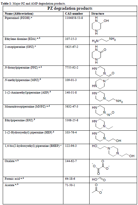
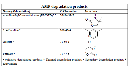
Table 1: Major PZ and AMP degradation products.
To measure organic acids and heat-stable salts, established techniques are utilized. However, the measurement of NVDPs using available chromatographic methods is still in the early stages of development.10-12 NVDPs, characterized by their low molecular weight, high volatility, high polarity, and high viscosity, are naturally basic and hydrophilic. Additionally, they exist in a solution with a high concentration of primary amines. These properties present significant challenges in terms of extraction and separation, and they can have a detrimental effect on general chromatographic materials.10
The measurement of NVDPs in PZ, AMP, and PZ/AMP blends was carried out using gas chromatography-mass spectrometry (GC-MS) and ion chromatography.8,9,12 However, these results were based on degradation under simulated conditions.13 Under operational conditions, results on the degradation products of MNPZ, DMOZD, OPZ, FPZ, EDA, and 2,4-lutidine were reported.6,14 Regrettably, there were no specifics provided regarding the analytical methods used. Overall, there is a dearth of information concerning measurement methods and result accuracy.11
2. Experimental
2.1 Apparatus
A liquid chromatography-triple quadrupole mass spectrometer (LC-MS/MS) was used for the analysis. This system consisted of a 1290 infinity II LC system with a 6-position/14-port valve multi-column thermostat coupled to a 6495C MS/MS with electrospray ionisation from Agilent Technologies (Santa Clara, CA, USA). Instrument control and data analysis were performed using Agilent MassHunter Workstation software. A Bransonic® Ultrasonic Bath 3800 (Brookfield, CT, USA) was employed as a water bath and for sonication and degassing of solvents and solvent mixtures. Mixing was conducted with a Lab Dancer Vortex Orbital Shaker from IKA-Werke (Staufen, Germany). pH measurements were carried out using a Metrohm (Herisau, Switzerland). Samples and reagents were weighed using a top-loading analytical balance, VWR LPG-4202i, from VWR International (Leuven, Belgium). Standards were weighed using a Sartorius MC 210 P from Sartorius (Göttingen, Germany). Adjustable pipettes from Thermo Fisher Scientific (Joensuu, Finland) were used to dispense volumes in the ranges 2-20 µL, 10-100 µL, and 100-1000 µL. Samples were filtered through 0.2 µm PTFE syringe filters from Agilent Technologies (Santa Clara, CA, USA) and processed in standard 15 mL centrifuge tubes. The samples were injected into standard 1.5 mL vials. Chromatographic separation was tested on various columns: Zorbax RRHD Eclipse Plus C18 (C18), 2.1 x 50 mm, 1.8 µm from Agilent Technologies (Santa Clara, CA, USA); Ascentis® Express C8 (C8), 4.6 x 150 mm, 2.7 µm; Discovery® HS F5 Pentafluorophenylpropyl (PFP), 2.1 x 150 mm, 3 µm; Ascentis® Express Phenyl-Hexyl (PH), 4.6 x 150 mm, 2.7 µm; Ascentis® Express ES-Cyano (CN), 4.6 x 100 mm, 2.7 µm; Ascentis® Express RP-Amide (RP-Amide), 4.6 x 50 mm,
2.7 µm from Merck KGaA (Darmstadt, Germany); and Hypercarb™ Porous Graphitic Carbon (PGC), 4.6 x 150 mm, 5 µm from Thermo Scientific.
2.2 Chemicals and Reagents
Acetonitrile and methanol of LC-MS quality were purchased from Merck KGaA (Darmstadt, Germany). Deionised water (18.2 MΩ·cm) was prepared in the laboratory using a Millipore Milli-Q system (Darmstadt, Germany). Ammonium formate and ammonium acetate of LC-MS quality were obtained from Sigma Aldrich (St. Louis, MO, USA), and formic acid was sourced from VWR International (Leuven, Belgium). Neat standards of 99.7% OPZ, 99.9% MPZ, and 99.6% BHEP were acquired from Sigma Aldrich (St. Louis, MO, USA). FPZ at 99.1% was purchased from Tokyo Chemical Industry (Tokyo, Japan), 97.0% DMOZD from Apollo Scientific (Stockport, UK), 99.8% HEP from Alfa Aesar (Lancashire, UK), 99.9% MNPZ from Chiron AS (Trondheim, Norway), 99.6% EDA from Merck KGaA (Darmstadt, Germany), and 99.4% 2,4-lutidine from Thermo Fisher Scientific (Geel, Belgium). Stock solutions of 10,000 µg·mL⁻¹ were prepared in various solvents and working standard mixtures of 1,000 µg·mL⁻¹ and 100 µg·mL⁻¹ were prepared in acetonitrile. Deuterated MNPZ (MNPZ-d8) with a purity of 95.0% was purchased from Chiron AS (Trondheim, Norway) at 100 µg/mL to be used as an internal standard. It was diluted to a working standard solution of 1 µg·mL⁻¹ in acetonitrile. A blank solution of CESAR1 solvent was prepared by weighing approximately 130 g of 100% purity PZ from Sigma Aldrich (St. Louis, MO, USA) and approximately 270 g of 99.6% purity AMP from Merck KGaA (Darmstadt, Germany) into a 1000 mL HDPE volumetric flask. Deionised water was added to the mark after all the salt had dissolved.
2.3 Method development, validation and application
The general scheme in Figure 1 was used for the development, validation and application of the method.
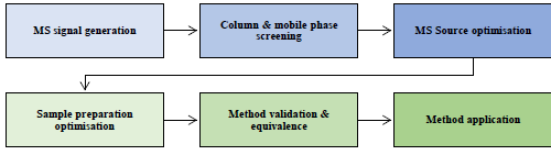
Figure 1: General method development process applied.
2.4 MS signal generation
For the analysis using the Agilent MassHunter Optimizer software, pure standards were diluted with a mobile phase composed of 0.1% formic acid in a 50:50 mixture of water and methanol to achieve a concentration of 0.1 µg·mL-1. Each standard was then injected into the LC-MS system using flow injection and a C18 column via autosampler. The collision energy (CE) was scanned from 0 to 80 V and the scanned precursor ions were [+H] and [+NH4]. A maximum of four product ions was determined with a low mass cut-off of 30 m/z. The optimization conditions included capillary and nozzle voltages of 500 V and 300 V, a drying gas flow of 15 L·min-1 at 230 °C, a sheath gas flow of 8 L·min-1 at 400 °C, and a nebulizer pressure of 15 Psi with a constant fragmentor voltage of 166 V.
2.5 Column and mobile phase screening
In order to select the most suitable column and mobile phase for our analysis, we conducted a thorough screening process. We prepared each standard at a concentration of 0.1 µg·mL-1 and injected them into various RP columns (C18, C8, PGC, PFP, PH, RP-Amide, and CN) using different compositions and ratios of the mobile phase. We tested aqueous solutions of water, 0.1% formic acid in water, 6 mM and 12 mM ammonium acetate, and ammonium formate in different ratios to the organic solvent. Additionally, we used methanol, 0.1% formic acid in methanol, and acetonitrile as the organic composition of the mobile phase in isocratic mode. The retention factor (k) was calculated with a target value between 1-5. We also tested the OH5 and CN columns in HILIC mode with acetonitrile as the organic phase. The final selection of the column and mobile phase was based on achieving acceptable retention factors for a large number of analytes in a single method with optimal selectivity between the analytes and the main amines.
2.6 MS source optimisation
Once the column and mobile phase were selected, we used them as the base method to create a dynamic multiple- reaction monitoring method with one transition per molecule. The Agilent MassHunter Workstation Source Optimiser was then used to optimize ion funnel voltages, gas temperatures and flows, nebulizer pressure, capillary voltage, and nozzle voltage using the “One Factor at a Time” (OFAT) approach.
2.7 Sample Preparation Optimization
In addition, we utilized a Resolution III screening design to optimize the sample preparation process. This involved investigating the influence of different factors and their interactions on the quantification of the sample. We utilized a screening design with seven factors and two levels, generated using Statgraphics® Centurion 18. The peak areas of the prepared sample were selected as the experimental response with the aim of maximization. We also performed a thorough check for the identification of degradation products and confirmation of the results by checking the blank response to detect the formation of artefacts, ensuring a difference of ± 0.1 min between the retention time of the degradation product in the sample and the standard, and verifying the presence of two fragment ions and an ion ratio within ± 30%. Table 2 shows the parameters analyzed and their ranges. Identified significant variables were later analyzed one factor at a time.15,16
Table 2: Design parameters of the factors that could influence the instrumental determination of NVDP.
| Experimental factor | Units | Variable type | Low factor level (-) | High factor level (+) |
| Mass of sample | g | continuous | 0.25 | 0.5 |
| Extraction solvent | – | categorical | methanol | water |
| pH of extraction solvent | – | continuous | 3 | 7 |
| Extraction solvent ratio | – | continuous | 1 | 10 |
| Vortex time | minutes | continuous | 1 | 5 |
| Injection solvent | – | categorical | methanol | aqueous mobile phase |
| Column temperature | °C | continuous | 25 | 35 |
2.8 Sample preparation
The samples, stored in 30 mL HDPE bottles, underwent a meticulous preparation process. Initially, the samples were equilibrated in a water bath at 45°C for thirty minutes, with regular shaking every ten minutes to ensure thorough mixing and dissolution of any precipitated PZ.5 Subsequently, the samples were allowed to equilibrate at room temperature for one hour and then mixed ten times by inverting to achieve homogeneity. The homogenized samples were then filtered through a 0.2 µm PTFE syringe filter, effectively removing any suspended particles in the solution.
2.9 Extraction and Partitioning
To extract the analytical portion, a 15 mL centrifuge tube was utilized as the container. The extraction solvent was carefully added to the analytical portion, and the container was sealed with a cap. The vortex was employed to shake the mixture, with specific attention given to the extraction solvent, the sample-to-solvent ratio, and the shaking time, which were all meticulously analyzed.11
2.10 Calibration solutions
Prior to calibration, individual standard solutions (Ri) were prepared in six replicates at 0.1 µg·mL-1 and compared with the detector response of the same standards in a mixed solution (Rm) at the same concentration. The comparison determines whether the detector response of the individual standards is affected when the standards are mixed for a multi-standard calibration. The effect of mixing standards on the calibration (EMC) was calculated using the adopted relationship [EMC= ((𝑅𝑅𝑚𝑚⁄𝑅𝑅𝑖𝑖) − 1) × 100)].16 The effect is considered significant for a standard if it leads to a deviation of more than ±10 %. Matrix effects (ME) were compared by comparing the slope of the prepared calibration standards in the blank CESAR1 solvent (matrix-matched slope, Sm) and in the solvent (Ss). The effect on the signal compared by the relationship [ME= ((𝑆𝑆𝑚𝑚⁄𝑆𝑆𝑖𝑖 ) − 1) × 100)]. The effects were considered significant if they were greater than ±20 %16. The linearity and range were determined from 0- 150 % of the highest MNPZ concentration in the ALIGN-CCUS campaign, 5- 5000 ng·mL-1.17
2.11 Fortifications
For recovery studies, a precise volume of standard solutions at the desired concentration was added to a weighed CESAR1 blank sample. The fortified sample underwent thorough mixing for 30 seconds using a vortex. Subsequently, the sample was allowed to stand for approximately five minutes to ensure even distribution of degradation products and their interaction with the matrix.
2.12 LC-MS analysis
The LC-MS analysis involved the use of a carefully selected column and optimized source conditions. The flow rate and injection volume were specifically tailored to the column dimensions and analyte response. To ensure accurate results, time segments were employed to divert highly concentrated main amines away from the mass spectrometer. Additionally, an isotopically labelled MNPZ-d8 was used as an injection internal standard (I-IS) at a concentration of 30 ng·mL-1 in the calibration standards and the final extract of each sample. The I-IS played a crucial role in minimizing biases resulting from injection errors and matrix effects.16
To quantify and report an identified degradation product in the sample, the following criteria needed to be met:15,16
- The retention time should differ by no more than ± 0.1 minutes from that of a standard with a similar concentration.
- Two transitions (qualifier and quantifier product ions) were required, and the ratio of the transitions needed to fall within ± 30%.
- The recovery result of the fortified samples had to be within the expected range based on concentration.
- The linearity parameter R2 needed to be greater than or equal to 0.995.
2.13 Method validation, equivalence and application
The method validation process involved thorough examination of various parameters to ensure the reliability and accuracy of the final sample preparation method. This included evaluating selectivity, linearity, limit of detection (LOD), limit of quantification (LOQ), accuracy, repeatability, and measurement uncertainty.15,16,18 Selectivity was assessed by analyzing the response of target molecules in blank samples and specific qualifier and quantifier ions. The LOD and LOQ were determined from the calibration curve parameters using the three lowest calibration levels.19 The LOQ was set as the lowest fortification level that met the performance criteria of the method. Accuracy was evaluated through recovery and expressed as relative bias, while repeatability was assessed as relative standard deviation. Measurement uncertainty was determined from the validation data using the bias and repeatability components.15,16,18
Furthermore, method equivalence was established by comparing TCM LC-MS results with those obtained by SINTEF industrial laboratories during the 2019/2020 campaign. Hypothesis tests were conducted using a t-test to compare mean values, regression line analysis to cover the linear range, and the non-parametric Wilcoxon signed-rank test to validate the parametric assumption of previous tests. The results were used to assess the stability of degradation products during storage and, if stable, to perform method equivalence studies. Finally, the validated method was applied to real samples from the 2019/2020 ALIGN-CCUS campaign, which were stored at 5°C in high-density polyethylene (HDPE) containers.20,15
3 Results and discussion
3.1 MS signal optimization
In the positive ionization mode, all molecules were ionized with the protonated molecule [M+H]+. The optimization process automatically adjusted the corresponding transitions and fine-tuned the collision energies, maintaining a constant fragmentor voltage of 166 V. We used the multiple reaction monitoring (MRM) transition with the highest abundance for quantification and the second highest for qualification. In cases where two transitions had comparable abundance, we selected the transition with the higher molecular mass to minimize spectral and matrix-related interference effects. The detailed results can be found in Table 3. Given the close pKa values of NVDPs and the main amines, as well as the high concentration of the main amines in the samples, we optimized PZ and AMP to ensure that the selectivity experiments were conducted at a controlled concentration. This approach was adopted to manage the separation, prevent detector saturation, and minimize alterations to the column chemistry.
Table 3: pKa, Transitions and corresponding collision energies (CE) at a fragmentor voltage of 166 V selected for analysing NVDPs in CESAR1 solvent using ESI in the LC-MS/MS system.
| Compound | pKa | precursor ion | quantifier ion (CEa) | qualifier ion (CEa) |
| FPZ | 8.58 | 115.1 | 87.2 (8) | 44.4 (24) |
| DMOZD | 12.91 | 116.07 | 72.2 (12) | 55.2 (16) |
| OPZ | 15.47 | 101.07 | 72.2 (12) | 44.3 (20) |
| MPZ | 4.94/9.09 | 101.11 | 58.2 (24) | 44.3 (24) |
| BHEP | 14.96 | 175.15 | 88.1 (20) | 45.3 (36) |
| HEP | 14.66 | 131.12 | 88.1 (16) | 44.3 (32) |
| MNPZ | 8.07 | 116.08 | 86.2 (4) | 56.2 (20) |
| EDA | 10.71 | 61.08 | 44.3 (8) | 29.3 (76) |
| 2,4-Lutidine | 6.99 | 108.08 | 92.1 (24) | 65.2 (28) |
| PZb | 9.73 | 87.1 | 44.3 (20) | 30.3 (60) |
| AMPb | 12.91/9.7 | 90.1 | 55.2 (16) | 45.3 (24) |
| MNPZ-d8 | ̶ | 124.13 | 94.2 (4) | 62.2 (24) |
a is the Collision Energy associated with the ion in volts.
b These were only used for the preliminary selectivity studies.
3.2 Column and mobile phase screening
Among the columns tested, PGC and PFP showed the best selectivity for NVDPs compared to the main amines. C8, C18, CN, and PH were only able to retain DMOZD using a low solvent strength mobile phase. It is possible that “dewetting” of the stationary phase occurred. The elution order and selectivity are presented in Figure 2.21
The PGC column, designated as method one, showed adequate retention of most analytes at a pH of about seven. There was adequate separation with NVDP eluting at retention times between the two main amines using a mobile phase of 12 mM ammonium acetate: methanol (50:50 % v/v) in isocratic mode. HEP, BHEP, FPZ, MNPZ, and MPZ eluted between the two main amines of AMP and PZ at an injection volume of 2.5 µL, a flow rate of 1.0 mL·min-1
and a run time of 27 minutes. The polarizable PGC surface could contribute to charge induction and retention of polar compounds, while the flat surface could be partially responsible for the resolution of closely related structures. Although OPZ, EDA, and DMOZD were retained by PGC, OPZ coeluted with AMP, while EDA coeluted with PZ, resulting in interfering matrix effects. Spectral interference occurred between DMOZD and MNPZ so they could not be determined by one method. The PGC column did not retain 2,4-lutidine.22,23 On the other hand, PFP showed controlled retention and different selectivity when the composition of the mobile phase was systematically changed. At a pH of about seven, OPZ and DMOZD eluted earlier than a non-separated peak of AMP and PZ when 12 mM ammonium acetate: methanol (50:50 % v/v) was used as the mobile phase in isocratic elution. An injection volume of 5.0 µL, a flow rate of 0.3 mL·min-1 and a run time of 15 minutes were used. This was referred to as method two. This suitability was chosen because in addition to the spectral interference between DMOZD and MNPZ, MNPZ and EDA were also coeluted with PZ, resulting in matrix interference. The elution order and separation can be explained by the predominant ion-exchange retention mechanism of the basic analytes, while non-ionic retention mechanisms could explain the significant selectivity differences between the analytes.24
At a pH of about seven, neither PGC nor PFP columns retained 2,4-lutidine. This could perhaps be due to its lower pKa value (6.99), so that it was in a non-ionised form. This could mean that the polarisability on the PGC surface was no longer present and the ion exchange mechanisms prevalent in the PFP phase are ineffective. To overcome this, method three was tested in which 2,4-lutidine was eluted after the main amines of AMP and PZ, respectively, at a pH of approximately three. The separation was performed using the PFP phase and a mobile phase consisting of 0.1 % formic acid in water: methanol (75:25 % v/v) in isocratic mode. An injection volume of 2.0 µL, a flow rate of 0.3 mL·min-1 and a run time of 15 minutes were used. This pH was lower than the pKa of 2,4-lutidine and was therefore ionised, allowing the use of the ion-exchange retention mechanism of the PFP phase. At this pH, EDA coeluted with PZ, while only FPZ and DMOZD were retained by the PGC phase. The coelution of PZ and EDA could be because the two nitrogen atoms are the predominant active sites in EDA and there are no other predominant analyte-column interactions.21
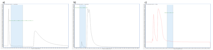
Figure 2: Elution and retention of degradation products in relation to the main amines. The blue highlight shows the elution zone of NVDP of interest. The three methods showed different retentions for a) HEP, BHEP, FPZ, MNPZ and MPZ, all eluted between AMP and PZ in method one, using Hypercarb™ PGC (4.6 × 150 mm, 3 µm), b) OPZ and DMOZD, which were eluted in the second method using Discovery® HS F5 PFP (2.1 × 150 mm, 3 µm) and c) 2,4-lutidine, which was eluted after the AMP and PZ peaks using Discovery® HS F5 PFP (2.1 × 150 mm, 3 µm). In the final dMRM methods, the main amines were diverted to waste to avoid saturation of the detector.
3.3 MS source optimisation
The performance of a mass spectrometer (MS) can be significantly impacted by the efficiency of ion transmission from the source to the MS, which in turn affects the sensitivity and signal intensity of different molecules. Various factors come into play in optimizing this process. For instance, the nebulizer pressure, temperature, and flow rate of the drying gas and sheath gas are influenced by the flow rate of the liquid chromatography (LC) system. Additionally, the ion funnel voltage, capillary voltage, sheath gas temperature, and nozzle voltage are dependent on the specific molecular properties. For more detailed information, please refer to Table 4 for the results.
Table 4: Optimised MS source conditions for the analysis of NVDPs in CESAR1 solvent.
| Parameter | Method one | result Method two | Method three |
| HPRF a voltage (V) | 130 | 130 | 210 |
| LPRF b voltage (V) | 40 | 60 | 60 |
| Sheath gas temperature (°C) | 400 | 400 | 400 |
| Sheath gas flow (Litres/ min) | 12 | 10 | 12 |
| Gas temperature (°C) | 230 | 170 | 110 |
| Gas flow (Litres/ min) | 17 | 13 | 11 |
| Nebulizer (psi) | 40 | 60 | 20 |
| Capillary voltage (V) | 2000 | 2000 | 1000 |
| Nozzle voltage (V) | 500 | 0 | 0 |
a High-pressure Ion funnel radio frequency.
b Low-pressure Ion funnel radio frequency.
3.4 Sample Preparation Optimization
When the dilution factor was appropriately scaled, the sample size did not significantly affect the quantification of NVDPs. However, a higher sample-to-solvent ratio seemed beneficial, possibly due to the larger volume available for distribution. At a dilution factor of 1000, the extraction of a 0.5 g sample in 5 mL solvent (1:10 ratio) and dilution to 1000 µL in vials (1:100 ratio) was found to be better than the extraction of 0.5 g in 0.5 mL solvent (1:1 ratio) and dilution to 1000 µL in vials (1:1000 ratio).
NVDPs extraction was tested at one, three, five, seven, and ten minutes of shaking with a vortex. The concentration of MNPZ, MPZ, and FPZ peaked at three minutes (Figure 3). Therefore, four minutes was set as the standard extraction time for all methods. Although initial analysis suggested that the low pH (about three) of the extraction solvent and methanol was significant, further evaluation indicated that the high observed response was due to the formation of artefacts of FPZ, MPZ, and MNPZ.
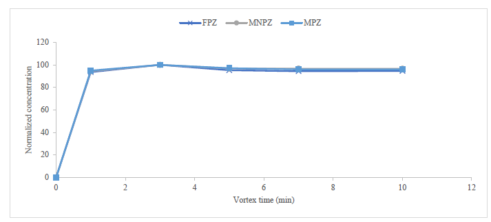
Figure 3: Influence of vortex time on the amount of degradation product determined. The normalised concentration is plotted against the vortex time to eliminate the influence of the actual concentration value.
At a low extraction pH, the high added concentration of formic acid additive could have led to the formation of FPZ.6,14 The presence of MNPZ could be attributed to nitrosation when an acidified extraction solvent was used.9 This occurrence was not observed when the pH of the aqueous injection solution was adjusted to around five. The use of methanol and acidified methanol for extraction may have led to the formation of MPZ and MNPZ artefacts through alkylation25,26 potentially OH-initiated nitrosation.27 Extraction with water without pH adjustment was standardized for all methods. To preserve the integrity of the silicate-based PFP column, the pH of the injection solution was adjusted to around five using 0.015% formic acid for methods one and two. In method three, 0.1% formic acid was adequate to achieve a final pH of approximately five, which was below the pKa of 2,4-lutidine.
These measures ensured that the pH of the injection solution remained within the operational limits of the silica-based PFP phase, preventing the formation of artefacts. Matching the mobile phase and injection solution guaranteed that the methods produced good and acceptable peaks.28,29 Column temperature did not significantly affect the quantified amount of degradation products. However, higher temperatures led to unacceptable retention times concerning the void volume for early eluting degradation products.15 The column temperature was maintained at 25 ±2°C. Table 5 details the final method protocol used during method validation and application.
Table 5: Method protocol for the measurement of NVDPs In CESAR1 solvent.
| Step | Procedure |
| 0 | Place the samples in a liquid water bath at 45 °C for 30 minutes and shake them by hand every 10 minutes. Allow the samples to equilibrate for one hour at room temperature. Homogenise the sample by inverting 10 times. |
| 1 | Filter sample through 0.2 µm pore size and transfer 0.5 g of an analytical portion into a 15 mL centrifuge tube. |
| 2 | Add 4.5 mL of deionised water. |
| 3 | Shake by vortex for four minutes. |
| 4 | For methods one and two, take 10 µL of the sample and add it to a vial containing 960 µL of diluent (12 mM ammonium acetate with 0.015% formic acid) and 30 µL of the IS. Inject into the LC−MS module. For method three, take 10 µL of the sample and add it to a vial containing 960 µL of diluent (0.1% formic acid: methanol 75:25% v/v) and 30 µL of the IS. Inject into the LC−MS module. |
3.5 Method validation
The validation process involved testing all molecules at three different concentration levels: the target LOQ level of 10 ug.Kg-1, mid-level, and high-level concentrations. However, MNPZ was an exception as it was only validated at 100 ug.Kg-1 due to being purchased pre-diluted at a low concentration. The accuracy, repeatability, and expanded uncertainty assessments demonstrate that the method of analysis is reliable and meets the acceptable guidelines as outlined in the references.15-18,30 For detailed results of the validation, please refer to Table 6 below.
Table 6: Summary of the method validation results for the analysis of NVDPs in CESAR1 solvent using LC-MS/MS.
| Degradation compound | Instrumental limits | Validation level | Accuracy | Repeatability | Expanded uncertainty | |
| LOD (ug·Kg-1) | LOQ (ug·Kg-1) | Concentration (ug·Kg-1) a | Relative bias (%) | Relative standard deviation (%) | U (K=2) (%) | |
| FPZ | 3.36 | 10.07 | 10 | -1.70 | 10.56 | 28.57 |
| 500 | 0.18 | 6.37 | 17.26 | |||
| 4000 | 4.71 | 3.10 | 12.75 | |||
| MPZ | 1.71 | 5.12 | 10 | 0.48 | 2.37 | 6.50 |
| 500 | 3.26 | 5.07 | 15.58 | |||
| 4000 | -0.92 | 2.87 | 7.96 | |||
| MNPZ d | 5.93 | 17.78 | 100 | -10.88 | 2.46 | 22.67 |
| HEP | 0.74 | 2.23 | 10 | 14.39 | 8.75 | 38.34 |
| 500 | 8.40 | 2.97 | 18.77 | |||
| 4000 | -0.34 | 3.33 | 9.02 | |||
| BHEP | 2.39 | 7.17 | 10 | -1.65 | 3.61 | 10.25 |
| 500 | 7.35 | 6.64 | 23.70 | |||
| 4000 | -6.43 | 5.57 | 19.48 | |||
| DMOZD | 2.46 | 7.39 | 10 | 1.03 | 4.25 | 12.09 |
| 300 | -9.75 | 3.30 | 21.39 | |||
| 2500 | -6.51 | 5.38 | 19.52 | |||
| OPZ | 0.88 | 2.65 | 10 | -0.08 | 5.32 | 14.83 |
| 300 | -12.92 | 3.24 | 27.20 | |||
| 2500 | 0.37 | 5.50 | 15.39 | |||
| 2,4 Lutidine | 1.40 | 4.19 | 10 | -10.17 | 4.68 | 23.85 |
| 300 | -0.63 | 3.83 | 10.72 | |||
| 2500 | -12.49 | 5.21 | 30.35 |
d for a 1000-fold diluted sample, the concentration corresponds to mg·Kg-1 in the sample
As shown in Figure 4, the comparative evaluation showed agreement of the developed methods with the methods of the service provider using three complementary statistical tests.
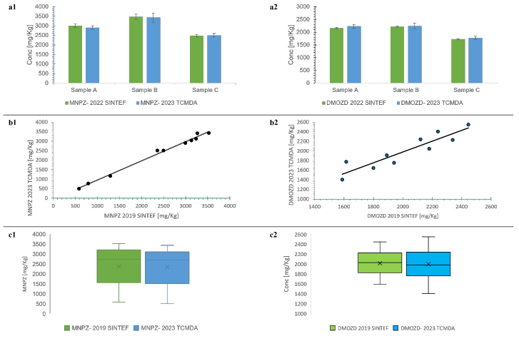
Figure 4: Method equivalence tests that show the comparability of the developed methods with the methods of the service provider. The “a” figures show the results of the t-test. The two methods were not significantly different at the concentrations tested (a1 MNPZ: Sample A: P (|t|≥2.20) = 0.05; Sample B: P (|t|≥0.35) = 0.73; Sample C: P (|t|≥0.63) = 0.54, and a2 DMOZD: Sample A: P (|t|≥2.16) = 0.08; Sample B: P (|t|≥0.71) = 0.51; Sample C: P (|t|≥1.63) = 0.15; at α= 0.05). The “b” figures show the results of the linear model. The two methods did not differ significantly over the entire measurement range (b1 MNPZ: intercept: P (|t|≥0.61) =0.56; slope: P (|t|≥0.31) = 0.77, and b2 DMOZD: P (|t|≥0.77) = 0.46; slope: P (|t|≥0.72) = 0.49 at α= 0.05). While the “c” figures show the results of the Wilcoxon signed-rank test. There was no statistically significant difference between the results obtained using the methods of the two laboratories (c1 MNPZ: W=20 ≥ 8 (test statistic), and c2 DMOZD: W=22 ≥ 8 (test statistic) at α= 0.05).19, 20
3.7 Method application
Ten samples from the ALIGN-CCUS campaign conducted in 2019/2020 were analysed using the newly developed methods. The samples represented the development of the matrix during more than 1200 hours of operation under different test conditions.5,6 The results presented in Figure 5 show that the samples contained five of the eight degradation products analysed, with 2,4-lutidine, HEP and BHEP below the LOQ equivalent of 10 mg·Kg-1. Additionally, PZ and MPZ, which were previously suspected but not quantified, were detected in the samples.5, 6 The validity of these findings was confirmed by the retention time falling within ± 0.1 min, two transitions, the ratio of transitions within ± 30 %, recovery results of the quality control (QC) sample at the LOQ (70−120 %), and linearity (R2 ≥ 0.995).15,16 These results affirm the efficacy of the developed methods in monitoring the degradation of CESAR1 for NVDPs.
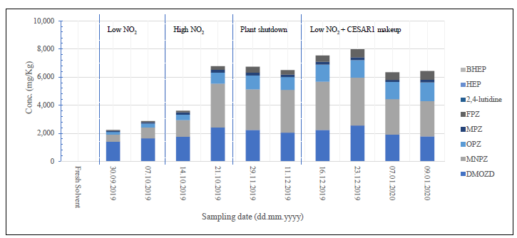
Figure 5: Results of aged CESAR1 solvent from the 2019/2020 ALIGN-CCUS campaign using the developed methods. The results show an increase in solvent degradation at high NO2 concentrations in the flue gas. As expected, solvent degradation decreased during a plant shutdown and increased again after start-up. The addition of fresh solvent diluted the degradation products. BHEP, HEP and 2,4-lutidine were below the LOQ (10 mg.Kg-1). All targeted degradation products were below the LOQ in the fresh solvent. Details on the operation of the plant are published in papers.2,5,6
3.8 Analyte stability of some NVDPs
The concentration of DMOZD, MNPZ, and 2,4-lutidine remained stable throughout the storage period. However, there was a significant decrease in the concentration of OPZ, ranging from 35% to 54% over the three-year period, as illustrated in Figure 6. Further analysis is required to ascertain the reason behind this decline. It is plausible that OPZ underwent degradation or transformation.
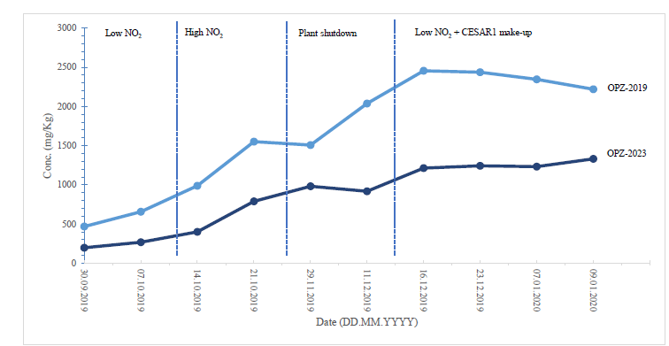
Figure 6: Comparison of results between SINTEF 2019 and TCM 2023 for OPZ with losses between 35- 54 %.
4. Conclusion
Our study validates the effectiveness of using LC-MS/MS for the ex-situ quantification of non-volatile degradation products (NVDPs) of solvents in the context of amine-based carbon capture process. We found that the stationary phases PGC and PFP were effective in separating most cyclic NVDPs from the primary amines using standard LC- MS/MS compatible solvents in isocratic mode. The separation of linearly structured NVDPs proved challenging in the reverse phase and requires further investigation. Our identification of previously unmonitored NVDPs in substantial quantities indicates the need to broaden the scope of analytes to be monitored. This may be achievable through simultaneous or combined target and non-target analyses.31,32 We also observed the loss of some degradation products with prolonged storage, which may impact sample stability and preservation, as well as the use of aged solvents for carbon capture.11
The availability of high-precision instrumentation on-site could greatly benefit carbon capture facilities. LC-MS/MS can effectively monitor NVDPs in solvents, absorber water, acid washes, and absorber emissions captured in solutions or filters in near real-time. It can serve as a complementary technique to inline online and at-line processes analysers.4
5. Acknowledgements
The authors express their sincere gratitude to TCMDA, Gassnova, Equinor, Shell, and TotalEnergies for their contributions and efforts toward this research. We also acknowledge the support provided by the Erasmus+ programme of the European Union through the EMQAL program, along with the Department of Chemistry at the University of Bergen (UiB).
6. References
- a International Energy Agency Greenhouse Gas R&D Programme (IEAGHG) Further Assessment of
Emerging CO2 Capture Technologies for the Power Sector and their Potential to Reduce Costs; IEAGHG:
Cheltenham, UK, September 2019. b Feron, P. & Cousins, Ashleigh & Jiang, Kaiqi & Zhai, Rongrong & Garcia,
Monica, 2020. An update of the benchmark post-combustion CO2-capture technology. Fuel. 273. 117776.
10.1016/j.fuel.2020.117776. c Garcia, S., et.al., Process Integration of Advanced Amine-based Solvents in Power and Industrial Plants: A New Benchmark for Post-combustion Carbon Capture? (March 31, 2021). Proceedings of the 15th Greenhouse Gas Control Technologies Conference 15-18 March 2021, Available at SSRN: https://ssrn.com/abstract=3816508 or http://dx.doi.org/10.2139/ssrn.3816508 - Hume, S. A.; Shah, M. I.; Lombardo, G.; Kleppe, E. R. In Results from Cesar-1 Testing with Combined
Heat and Power (CHP) Flue Gas at the CO2 Technology Centre Mongstad, TCCS–11. CO2 Capture, Transport and Storage. Trondheim 22nd–23rd June 2021. Short Papers from the 11th International Trondheim CCS Conference, SINTEF Academic Press: 2021. - Languille, B.; Drageset, A.; Mikoviny, T.; Zardin, E.; Benquet, C.; Ullestad, Ø.; Aronson, M.; Kleppe,
E. R.; Wisthaler, A., Atmospheric emissions of amino-methyl-propanol, piperazine and their degradation products during the 2019-20 ALIGN-CCUS campaign at the Technology Centre Mongstad. In The 15th Greenhouse Gas Control Technologies Conference (GHGT-15), 2021. - Languille, B.; Drageset, A.; Mikoviny, T.; Zardin, E.; Benquet, C.; Ullestad, Ø.; Aronson, M.; Kleppe,
E. R.; Wisthaler, A. In Best practices for the measurement of 2-amino-2-methyl-1-propanol, piperazine and their degradation products in amine plant emissions, Proceedings of the 15th Greenhouse Gas Control Technologies Conference, 2021; pp 15-18. - Benquet, C.; Knarvik, A. B. N.; Gjernes, E.; Hvidsten, O. A.; Romslo Kleppe, E.; Akhter, S. In First
process results and operational experience with CESAR1 solvent at TCM with high capture rates (ALIGN-CCUS
project), The 15th Greenhouse Gas Control Technologies Conference (GHGT-15), Abu Dhabi, 15-18 March; Abu Dhabi, 2021. - Campbell, M.; Akhter, S.; Knarvik, A.; Muhammad, Z.; Wakaa, A., CESAR1 solvent degradation and
thermal reclaiming results from TCM testing. In The 16th Greenhouse Gas Control Technologies Conference 2022 (GHGT-16), Lyon, France, 2022. - Gouedard, C.; Picq, D.; Launay, F.; Carrette, P. L., Amine degradation in CO2 capture. I. A review.
International Journal of Greenhouse Gas Control 2012, 10, 244-270. - Freeman, S. A. Thermal degradation and oxidation of aqueous piperazine for CO2 capture. University of
Texas at Austin, 2011. - Wang, T. Degradation of Aqueous 2-Amino-2-methyl-1-propanol for CO2 Capture. Telemark University
College, 2013. - Reynolds, A. J.; Verheyen, T. V.; Meuleman, E., 16 – Degradation of amine-based solvents. In AbsorptionBased Post-combustion Capture of CO2, Feron, P. H. M., Ed. Woodhead Publishing: 2016; pp 399-423.
- Cuccia, L.; Dugay, J.; Bontemps, D.; Louis-Louisy, M.; Vial, J., Analytical methods for the monitoring of
post-combustion CO2 capture process using amine solvents: A review. International Journal of Greenhouse Gas Control 2018, 72, 138-151. Electronic copy available at: https://ssrn.com/abstract=5024434 - Saeed, I. M.; Mazari, S. A.; Alaba, P.; Ali, B. S.; Jan, B. M.; Basirun, W. J.; Sani, Y. M.; Nizzamuddin,
S.; Mubarak, N. M., A review of gas chromatographic techniques for identification of aqueous amine degradation products in carbonated environments. Environmental Science and Pollution Research 2021, 28, 6324-6348. - Vevelstad, S. J.; Buvik, V.; Knuutila, H. K.; Grimstvedt, A.; da Silva, E. F., Important Aspects Regarding
the Chemical Stability of Aqueous Amine Solvents for CO2 Capture. Industrial & Engineering Chemistry Research 2022, 61 (43), 15737-15753. - Moser, P.; Wiechers, G.; Schmidt, S.; Figueiredo, R. V.; Skylogianni, E.; Monteiro, J. G. M.-S.,
Conclusions from 3 years of continuous capture plant operation without exchange of the AMP/PZ-based solvent at Niederaussem–Insights into solvent degradation management. In The 16th Greenhouse Gas Control Technologies (GHGT-16), IEAGHG: Lyon, France, 2022. - European Commission, 2002/657/EC: Commission Decision of 12 August 2002 implementing Council
Directive 96/23/EC concerning the performance of analytical methods and the interpretation of results (Text with EEA relevance) (notified under document number C(2002) 3044). European Commission, Ed. 2002. - European Commission Directorate-General for Health and Food Safety (SANTE), Analytical quality control
and method validation procedures for pesticide residues analysis in food and feed SANTE 11312/2021. DirectorateGeneral for Health and Food Safety: 2022. - Thompson, M.; Ellison, S. L. R.; Wood, R., Harmonized guidelines for single-laboratory validation of
methods of analysis (IUPAC Technical Report). Pure and Applied Chemistry 2002, 74 (5), 835-855. - Dr. Latimer, G. W., Jr. (ed.), Guidelines for Standard Method Performance Requirements. In Official
Methods of Analysis of AOAC INTERNATIONAL, 22 ed.; Dr. Latimer, G. W., Jr., Ed. Oxford University Press: New
York, 2023. - Konieczka, P.; Namiesnik, J., Quality assurance and quality control in the analytical chemical laboratory:
a practical approach. 2nd ed.; CRC Press Inc: Boca Raton, FL, USA, 2018. - Miller, J.; Miller, J. C., Statistics and Chemometrics for Analytical Chemistry. Pearson Education Limited:
2010; Vol. 6th. - Žuvela, P.; Skoczylas, M.; Jay Liu, J.; Ba̧ czek, T.; Kaliszan, R.; Wong, M. W.; Buszewski, B., Column
Characterization and Selection Systems in Reversed-Phase High-Performance Liquid Chromatography. Chemical reviews 2019, 119 (6), 3674-3729. - West, C.; Elfakir, C.; Lafosse, M., Porous graphitic carbon: a versatile stationary phase for liquid
chromatography. Journal of Chromatography A 2010, 1217 (19), 3201-3216. - Bapiro, T. E.; Richards, F. M.; Jodrell, D. I., Understanding the complexity of porous graphitic carbon (PGC)
chromatography: modulation of mobile-stationary phase interactions overcomes loss of retention and reduces variability. Analytical chemistry 2016, 88 (12), 6190-6194. - Bell, D. S.; Jones, A. D., Solute attributes and molecular interactions contributing to “U-shape” retention on
a fluorinated high-performance liquid chromatography stationary phase. Journal of Chromatography A 2005, 1073 (1-2), 99-109. - Lepaumier, H.; Picq, D.; Carrette, P.-L., New amines for CO2 capture. II. Oxidative degradation
mechanisms. Industrial & Engineering Chemistry Research 2009, 48 (20), 9068-9075. - Chen, W.; Fu, X.; Liu, X.; Ye, L.; Yuan, Y., Mechanistic insight into the photocatalytic N-alkylation of
piperazine with alcohols over TiO2 supported Pd catalysts. Molecular Catalysis 2023, 538, 112993.
Electronic copy available at: https://ssrn.com/abstract=5024434 - Tan, W.; Zhu, L.; Mikoviny, T.; Nielsen, C. J.; Wisthaler, A.; D’anna, B.; Antonsen, S.; Stenstrøm, Y.;
Farren, N. J.; Hamilton, J. F., Experimental and Theoretical Study of the OH-Initiated Degradation of Piperazine under
Simulated Atmospheric Conditions. The Journal of Physical Chemistry A 2020, 125 (1), 411-422. - Naidong, W.; Chen, Y.-L.; Shou, W.; Jiang, X., Importance of injection solution composition for LC–MS–
MS methods. Journal of pharmaceutical and biomedical analysis 2001, 26 (5-6), 753-767. - Wang, J.; Aubry, A.-F.; Cornelius, G.; Caporuscio, C.; Sleczka, B.; Ranasinghe, A.; Wang-Iverson, D.;
Olah, T.; Jemal, M., Importance of mobile phase and injection solvent selection during rapid method development and sample analysis in drug discovery bioanalysis illustrated using convenient multiplexed LC-MS/MS. Analytical methods 2010, 2 (4), 375-381. - Horwitz, W.; Albert, R., The Horwitz Ratio (HorRat): A Useful Index of Method Performance with Respect
to Precision. Journal of AOAC International 2006, 89 (4), 1095-1109. - Rajski, Ł.; Petromelidou, S.; Díaz-Galiano, F. J.; Ferrer, C.; Fernández-Alba, A. R., Improving the
simultaneous target and non-target analysis LC-amenable pesticide residues using high speed Orbitrap mass
spectrometry with combined multiple acquisition modes. Talanta 2021, 228, 122241. - García-Reyes, J. F.; Hernando, M. D.; Ferrer, C.; Molina-Díaz, A.; Fernández-Alba, A. R., Large scale
pesticide multiresidue methods in food combining liquid chromatography–time-of-flight mass spectrometry and tandem mass spectrometry. Analytical Chemistry 2007, 79 (19), 7308-7323
Demonstration of CO2 Capture Process Monitoring and Solvent Degradation Detection by Chemometrics at the Technology Centre Mongstad CO2 Capture Plant (2023)
Jayangi D. Wagaarachchige, Zulkifli Idris, Ayandeh Khatibzadeh, Audun Drageset, Klaus-J. Jens and Maths Halstensen
Abstract
Solvent management is one of the important current challenges in post combustion carbon capture (PCC) technology development. Using large-scale 1960 h test campaign data (Technology Centre Mongstad, Norway, 2015 MEA Test), we demonstrate a combination of multivariate methods (PLS-R, MSPC) and process analytical spectroscopy (FT-IR) as a tool to monitor and control PCC process performance. Two MEA solvent monitoring models, total inorganic carbon (TIC) content and total alkalinity (TA), were prepared. In long-term solvent monitoring, PLS-R model prediction uncertainty increased due to gradual solvent changes, e.g., solvent degradation and impurity accumulation. Hence, we show a specific model update methodology to keep the models updated, leading to good long-term monitoring ability of the TIC and TA models. In addition to reliable long-term solvent monitoring ability, a new principle for follow-up of thermal solvent reclaiming was demonstrated. This shows that the need for solvent reclaiming can be quantified. Furthermore, this methodology is an indicator to see the actual solvent deviation from the fresh solvent. This quantification may provide an input for “start” and “end of reclaiming operation” identification. Hence, we demonstrate that it is possible to extract information for process performance follow-up, solvent monitoring, and solvent reclaiming from a single spectroscopic instrument.

Keywords: Basicity Calibration Degradation Fourier transform infrared spectroscopy Solvents
This publication is licensed under CC-BY 4.0 .
Copyright © 2023 The Authors. Published by American Chemical Society
1. Introduction
The devastating environmental impacts of climate change are the biggest challenges of the 21st century. Post-combustion carbon capture (PCC) is an essential effort to eliminate the anthropogenic CO2 emissions from burning of fossil fuels. The gas–liquid absorption–desorption process is the most prevailing abatement technology available in the industry. The 30 wt % aqueous monoethanolamine (MEA) solution is considered a typical benchmark solvent for CO2 capture. (1) High energy penalty for solvent regeneration (2) corrosivity of the solvent, (3,4) high solvent losses due to oxidative and thermal degradations, (5−9) and environmental concerns due to possible emissions (10) are major issues that still need to be addressed for an effective operation of PCC.
In order to maintain optimal performance of the CO2 capture process, it needs to be monitored and controlled. The application of process analytical technology (PAT) using spectroscopy is an important approach for enhanced control of CO2 capture operations. Spectroscopy is a powerful non-invasive analytical technique for chemical analyses giving direct speciation measurements at molecular level. Partial least squares regression (PLS-R) is a valuable statistical method to extract quantitative chemical information from spectroscopic data. PLS-R models have been successfully used by us for online monitoring/speciation of MEA solvent-based CO2 capture. (11,12) Furthermore, preparation of Fourier-transform infrared (FTIR) spectroscopy-based PLS-R models for MEA solvent is published. (13−15) This contribution demonstrates application of PAT and spectroscopy for solvent degradation follow up exemplified by the use of available test campaign data of the TCM MEA2 campaign.
In terms of solvent management, spectroscopy is useful since it is sensitive to molecular change of the chemical system. PLS-R models are useful for extraction of specific chemical information of interest, for instance total solvent alkalinity, total inorganic carbon, etc. from spectroscopic data. These data are useful to give an early warning of upcoming chemical solvent change. As the solvent composition changes in service (i.e., solvent degradation and accumulation of flue gas impurities contents), the PLS-R model of the monitoring loop must be updated to stay representative for the state of the process. A deviation of the PLS-R model prediction parameters [i.e., Q-residual (Q) and Hotelling’s T2 (T2)] is an indication of a deviation between actual solvent state and fresh solvent. Multivariate statistical process control (MSPC) is a method that can be used in process control with the use of, e.g., PLS-R models diagnostic measures such as Q and T2. (16,17) Hence, suitable process control decisions for solvent management can be taken accordingly.
The Technology Centre Mongstad (TCM) is one of the largest global post-combustion CO2 capture test centers which holds the most advanced test arena for CO2 capture. Until now, several test campaigns using aqueous 30 wt % MEA solvent have been demonstrated and the outcomes from these campaigns have been published. (10,18−22) The University of South-Eastern Norway (USN) received a comprehensive data set of TCM’s 2015 campaign (MEA2) for chemometric evaluation.
This paper presents a FTIR-based PAT approach using PLS-R models for continuous process monitoring and solvent degradation detection in an amine-based CO2 capture plant using data from the TCM plant.
2. Materials and Methods
2.1. Materials
In this study, TCM-MEA2 campaign FTIR spectra and corresponding analytical data were utilized. All data used are off-line sample measurements that were obtained from the same sampling point (Lean stream) of the TCM Amine Plant located at Mongstad, Norway.
FTIR spectra of 125 samples were measured during the total campaign period using a Bruker ALPHA ATR-FTIR spectrometer with a diamond crystal and were used as input data to the PLS-R models. Furthermore, TCM provided the total inorganic carbon (TIC) and total alkalinity (TA) analysis data (reference data) that were recorded during the actual campaign period corresponding to the given spectra. The reference data were used as the response output variables of the PLS-R models that were prepared in this work. The details are shown in Table 1.
Table 1. Details of the Reference Data Used for the Preparation of Models (MEA2 Campaign)
| reference analysis method (10) | species group | reference analysis unit | number of reference data |
|---|---|---|---|
| total alkalinity | amine species | mol/kg | 103 |
| total inorganic carbon | CO2 species | mol/kg | 120 |
2.1.1. Origin of Data: The 2015 TCM-DA MEA2 Campaign
MEA2 is a 1960 h operation which started on 6th of July 2015 and lasted until 17th October, 2015. (10) The base case testing was performed on 7th September, 2015 in the steady state condition after approximately 8 weeks since startup. (18) Morken et al. illustrated the overall campaign operational hours, (10) whereas Gjernes et al. tabulated the overall test activities. (20) This operation was mainly conducted using a combined-cycle gas turbine-based combined-heat-and-power (CHP) plant flue gas that contains about 3.5% CO2. (20) Furthermore, a mixture of CHP and RFCC (residual fluidized catalytic cracker)/RFCC flue gas alone was used for a few days. (20) This work contributed to several TCM authored publications on aqueous MEA-based CO2 capture by covering solvent emissions and degradation, (10) corrosion, (21) and reclaiming. (19) Thermal reclaiming was performed for 92 h after 1830 (day 77) h of campaign operation. After the reclaiming process was completed, the operation continued for another 28 h. Hence, the MEA2 campaign mainly comprises of the primary stages of an amine-based CO2 capture plant operation.
2.2. Methods
Figure 1 lists the three key stages of the data analysis hierarchy employed in this work. Figure 2 illustrates the main chemometric activities in each stage which are listed in Figure 1─using PLS-R model of CO2 (TIC-1). The same approach was followed in the analysis work on the total alkalinity model (TA-1). All the abbreviations/statistical paraments used in this work are tabulated in Table 2.


Table 2. Abbreviations/Statistical Parameters Used in the Chemometric Study
| abbreviation/statistical parameter | standfor | description |
|---|---|---|
| PLS-R models | partial least regression models | prediction models prepared using NIPALS algorithm; input variable is a part of a FTIR spectrum; output variables are total inorganic content (TIC) and total alkalinity values (TA) |
| TIC-1 | initial model of TIC | initial prediction model prepared for TIC |
| TA-1 | initial model of TA | initial prediction model prepared for TA |
| TIC-2 | updated model of TIC | updated prediction model for TIC |
| TA-2 | updated model of TA | updated prediction model for TA |
| RMSEP | average model prediction error | used to compare the model predictability and to select optimum latent variables (LVs) |
| LVs | latent variables | indicate number of components of PLS-R models |
| Q residual (Q) | quantification of the spectral information which not utilized in the PLS-R model prediction | indicate unusual spectral changes. Increase of Q indicate the more altered solvent condition than the fresh solvent state |
| leverage | measure of the effect of a sample on a PLS-R model/distance of a sample from PLS-R model centre | used to find suitable samples to use in model updating |
| Hotelling’s T2 (T2) | measure of the distance of sample from the centre of PLS-R model | in principle leverage and Hotelling’s T2 indicate same meaning; Hotelling’s T2 (T2) values are the standard for MSPC statistics (stage 2) |
2.2.1. Stage 1: Preparation of the Initial Models (TIC-1 and TA-1)
As shown in Figure 1, Stage 1, PLS-R models for CO2 (TIC-1) and total alkalinity (TA-1) species groups were initially prepared. The PLS-R algorithm known as NIPALS (nonlinear iterative partial least squares) was used in the model preparation. (23,24) Campaign data gathered up to 15th August 2015 (approximately initial 600 h of operation) were selected for calibration and validation processes of the TIC-1 and TA-1 models. (10) This was done to select the samples representing the non-degraded/fresh solvent. The infrared (IR) vibration band assignment of the chemical species was used to ensure only relevant variable ranges were used in the modeling. The FTIR spectra were preprocessed using the baseline correction method called Whittaker filter to remove unwanted baseline variation. (25) The models were validated using an independent test data sets which were obtained from the same initial 600 h MEA2 operation. Average model prediction errors were calculated as residual Y-variance of prediction which are denoted as root mean square error of prediction (RMSEP) (eq 1). (23) The optimal number of latent variables (LVs) (23) in the models were selected to attain the lowest values of RMSEP. Then, the models (TIC-1 and TA-1) were used for the prediction of the complete set of spectra of the MEA2 campaign.
where i─no of samples; ypredicted─predicted value; and yreference─measured value.
2.2.2. Stage 2: Refining PLS-R Models to Handle a Degraded Solvent
During the second stage, important statistical parameters (23) of TIC-1 and TA-1 predictions, such as Q residuals (Q), Hotelling’s T2 (T2), and leverages were recorded to adopt the models to the degraded solvent. All the spectral samples of the MEA2 campaign were mapped in the plot of T2 versus Q which is an important tool in fault detection. Recorded prediction leverages were used to select new samples for the model updating step which is described in Section 2.2.3.2.
2.2.3. Stage 3: Applications of PLS-R Model’s Prediction Statistics for Degrading Solvent Monitoring and Management
In the third stage, three different chemometric approaches were explored to demonstrate how the PLS-R model statistical parameters can be used to update the model to stabilize predictions during the whole operation, and how the model residuals are useful for solvent management.
2.2.3.1. MSPC Demonstration
The plot of T2 versus Q of TIC-1 model is used for MSPC demonstration. Moreover, calculated Q were used to check the lack-of-fit of the models for the entire campaign period. All the results are discussed in Section 3.2.
2.2.3.2. Model Updating
TIC-1 and TA-1 models were improved for reliable long-term predictions. Here, TIC-1 and TA-1 models were converted to upgraded models (TIC-2 and TA-2) for a better predictions of in the degraded/changed solvent conditions using a calibration transfer method (26) called model updating (MUP). (27,28) In order to convert the models, a few new calibration samples were selected to describe the solvent degradation/change of the total campaign. These samples were selected using prediction leverage versus samples (time) plot, as shown in Figure 2 stage 2. These selected samples were formerly studied by visualization of spectra to identify the spectral quality of the samples, prior to incorporating them in the available models. The model updating approach comprises several iterations to arrive at properly updated prediction models (TIC-2 and TA-2). Section 3.3 discusses the results of model updating approach of TIC and TA models.
All data analysis were performed on the MATLAB platform using PLS Toolbox 8.6.2 software.
3. Results and Discussion
3.1. Preparation of Initial PLS-R Models
The use of authentic industrial data will make the PLS-R models more tolerant to the actual process variations by the assimilation of realistic dynamic process variations. In this work, initial PLS-R models (TIC-1 and TA-1) were prepared for the demonstration of the and solvent change detection and PLS-R model updating during long-term operation.
Spectral preprocessing is a significant step of PLS-R model calibration using spectroscopic data. To extract chemical species variation, specific IR bands (Figure 3) are selected to improve the ratio of signal-to-noise. Initially, all spectra were baseline-corrected using the Whittaker filter with Lambda and Rho at 1000 and 0.001, respectively. (25) The raw spectra and preprocessed spectra of the MEA2 campaign are shown in Figure 3a,b. Additionally, Figure 3b indicates the variable ranges used in the TIC (blue shade) and total alkalinity (red shade) models.

The preferred method for preparing a robust model is selection of the specific IR vibrational bands of the specific species/group to be investigated. Table 3 summarizes the main selected species, the corresponding IR bands selected for models, model variable ranges, and reference literature.
Table 3. PLS-R Model Species, Identified IR Bands, Corresponding Literature IR Bands, and Variable Ranges of the Models
| models | species | identified IR bands (cm–1) | corresponding literature IR bands (cm–1) | variable ranges of models (cm–1) |
|---|---|---|---|---|
| TIC | MEACOO– | 1562 (1) | 1568, (14,29) 1564 (30) | [1590–1467], [1407–1301] |
| 1486 (2) | 1486 (14,29) | |||
| 1320 (3) | 1322 (14) | |||
| CO32– | 1387 (4) | 1388, (14,30) 1386 (29) | ||
| HCO3– | 1362 (5) | 1360, (14,30) | ||
| total alkalinity | MEA | 1020 (6) | 1024 (14) | [1670–1590], [1113–944] |
| MEAH+ | 1638 (7) | 1634 (14) | ||
| 1067 (8) | 1069, (14) 1064, (30) 1066 (29) |
Two models (TIC-1 and TA-1) were calibrated with test set validation. The used number of samples are presented in Table 4. Figure 4a,b depict the measured versus predicted plots of TIC-1 and TA-1 models, respectively. These figures indicate that the regression line of the models (fit line: red color) sets very close to the targeted line (1:1 line: green color). Model performance indicators─model range, RMSEP, number of LVs used, and R2 predicted─are tabulated in Table 4.

Table 4. Calibration and Validation Details of the Models (TIC-1 and TA-1)
| model | number of samples | model range mol/kg | RMSEP mol/kg | LVs | R2 (pred) | |
|---|---|---|---|---|---|---|
| calibration set | validation set | |||||
| TIC-1 | 17 | 16 | 1.1–1.5 | 0.024264 | 1 | 0.977 |
| TA-1 | 13 | 13 | 4.5–5.2 | 0.039841 | 2 | 0.948 |
3.2. Follow-Up and Control of Solvent Reclaiming
Reclaiming is an important part of CO2 capture solvent management. Thermal solvent reclaiming has been practiced in the gas sweetening industry for a long time (31) and recommendations vary on the maximum allowable amount of degraded solvent/contaminants. (32) The end point of thermal reclaiming has also been connected to the reclaimer temperature. (33) In conclusion, a more detailed method for thermal reclaimer follow-up seems desirable. We assess MSPC as a potential concept for thermal reclaimer follow-up and control. MSPC is an effective concept to follow-up and control of solvent reclaiming. One of the pillars of MSPC is PLS-R models which contribute by effective extraction of the information about the solvent changes from spectroscopic data (i.e., FTIR). (23)
In this work, the T2 and Q statistics is made by mapping all T2 versus MEA2 campaign samples’ Q values of TIC-1 model predictions (Figure 5a). Furthermore, Q values of MEA2 samples were plotted versus the days of operation (Figure 5b). Figure 5a shows the process variations in the MEA2 operation. The blue shaded area holds the campaign samples which agree with solvent composition at the start of operation. The samples in the red shaded area indicate the samples deviating from the average of model population (fresh solvent condition). Increased Q values indicates increased deviation. In addition, the red dashed lines separate the 95% confidence level of Q and T2.

Figure 5a is a plot showing solvent degradation during the CO2 capture process. Figure 5b depicts that the deviation of the Q residual is drastically increasing after day 27. (Date: 23 August 2015; @around 800 h of operation). (10) This deviation of the Q residuals indicates the difference between the current solvent state and the fresh solvent. According to Morken et al., the day 27 sample consists of about 0.5 wt % of heat stable salts (HSS) based on MEA weight, 3000 mg/L of anionic IC species, and 30,000 mg/L of main amine degradation products. (10) The observations in the T2 and Q statistics (Figure 5a) agree hence with the campaign sample analytics result. Furthermore, the plot indicates that Qs of the sample recorded on the day 77 and onward decrease and finally closely resemble the calibration samples. Solvent reclaiming started on day 77 of the campaign corresponding to samples collected on 12th October 2015 at around 1852 operation hours. Furthermore, this implies that the T2 and Q statistics have the ability to detect/indicate sufficient time/extent of reclaiming of the degraded solvent.
According to Figure 5b, Q show an increasing trend in three different stages starting from mid of August 2015 until solvent reclaiming initiation on 12th October 2015. A similar trend was observed by Flø et al. by solvent viscosity measurements at two different temperatures (30 °C and 60 °C). (19) This observation demonstrates that physical solvent changes influence the solvent spectra and correlate with prediction residual spectra (Q residual). In addition, the variation of HSS concentrations displays a similar tendency. (10) Therefore, Qs are mimicking both the physical and chemical variations observed during the MEA2 campaign operation.
Although the initial PLS-R models are useful for MSPC, they must be updated during the time of operation for reliable online monitoring. In this case, the T2 and Q statistics are useful for detection of the time to update the corresponding model. The adaptation of PLS-R models for prediction of the degraded solvent system is described in the following section.
3.3. Preparation of Updated (TIC-2 and TA-2) Models
Industrial PAT applications will fail if not model adaptation is carried out during the long-term use. PLS-R model calibration transfer methods are selected consequently based on the nature of the changes in the measuring environment, i.e., chemical changes, physical changes, instrument changes, etc. An applicable model updating method for CO2 capture solvent degradation is discussed below.
Figure 6a,b illustrates the total campaign prediction models of TIC-1 and TA-1, respectively. These plots indicate that the prediction error (RMSEP) of the TIC-1 and TA-1 models are increased by 70 and 123%, respectively, as time passes. Increase of the RMSEPs suggest that these model predictions develop a higher uncertainty over time in operation. In this context, the initial calibration data set needs to be expanded to obtain stable predictions during the total campaign. In order to expand the calibration data set of the models, a sufficient number of new samples need to be integrated. This is an iterative trial-and-error method across the total run time. In selecting new samples for a model renewal, leverage or T2 values are helpful statistical parameters.

Proper sampling techniques are essential to minimize sampling uncertainties/errors. Furthermore, identification of new samples needs to be done carefully since the selected sample may have a higher tendency for being an outlier. Visual observation of raw spectra of the samples is commonly used in identifying erroneous spectra. In addition, corresponding reference values (e.g., species concentration) of the selected samples should be acquired.
TIC-1 and TA-1 models were improved by adding 9 and 8 new data, respectively. Prediction parameters of the initial models (TIC-1 and TA-1) and updated models (TIC-2 and TA-2) are tabulated in Table 5, which indicates that the RMSEPs of the updated models were reduced by about 50% compared to the initial models. In agreement with Figure 6c,d, the prediction slopes of the TIC-2 and TA-2 models are improved─0.992 and 0.957, respectively. The number of latent variables of the updated models are also limited to three components, implying that the models are more robust in the predictive nature.
Table 5. Initial Models and Updated Models’ Performance Statistics
| model parameters | TIC models | total alkalinity models | ||
|---|---|---|---|---|
| TIC-1 | TIC-2 | TA-1 | TA-2 | |
| RMSEP (mol/kg) | 0.0415 | 0.0206 | 0.0953 | 0.0514 |
| R2 (predicted) | 0.985 | 0.992 | 0.882 | 0.920 |
| LVs | 1 | 3 | 2 | 3 |
4. Conclusions
MEA speciation models from the Technology Centre Mongstad 2015 MEA 2 Test campaign were developed. On this basis, two MEA solvent monitoring models, total inorganic carbon (TIC) content and total alkalinity (TA), were prepared. In addition, the ability of the models to cope with ongoing solvent change during the test campaign was demonstrated by application of a specific model update methodology.
Finally, to the best of our knowledge, a new method for solvent monitoring and management has been discovered and demonstrated. The need for solvent reclaiming can be quantified by the combination of statistical TIC or TA prediction model residuals. This methodology also provides “start” and “end of reclaiming operation” identification.
Hence, we demonstrate using large scale test campaign data that it is possible to monitor and follow-up process performance including solvent reclaiming operation and solvent monitoring using a single spectroscopic instrument.
Further development work is in progress on the issue of reclaiming monitoring and optimization.
Author Information
- Corresponding Author
- Maths Halstensen – Department of Electrical, IT and Cybernetics, University of South-Eastern Norway, Kjølnes Ring 56, 3918 Porsgrunn, Norway; Email: Maths.Halstensen@usn.no
- Authors
- Jayangi D. Wagaarachchige – Department of Electrical, IT and Cybernetics, University of South-Eastern Norway, Kjølnes Ring 56, 3918 Porsgrunn, Norway;
 https://orcid.org/0000-0002-1544-7169
 - Zulkifli Idris – Department of Process, Energy and Environmental Technology, University of South-Eastern Norway, Kjølnes Ring 56, 3918 Porsgrunn, Norway; https://orcid.org/0000-0001-7905-9686
- Ayandeh Khatibzadeh – Department of Electrical, IT and Cybernetics, University of South-Eastern Norway, Kjølnes Ring 56, 3918 Porsgrunn, Norway
- Audun Drageset – Technology Center Mongstad (TCM-DA), 5954 Mongstad, Norway
- Klaus-J. Jens – Department of Process, Energy and Environmental Technology, University of South-Eastern Norway, Kjølnes Ring 56, 3918 Porsgrunn, Norway; https://orcid.org/0000-0002-9022-5603
- Jayangi D. Wagaarachchige – Department of Electrical, IT and Cybernetics, University of South-Eastern Norway, Kjølnes Ring 56, 3918 Porsgrunn, Norway;
- Author ContributionsThe manuscript was written through contributions of all authors. All authors have given approval to the final version of the manuscript.
- FundingThis work was funded by the Ministry of Education and Research of the Norwegian Government.
- NotesThe authors declare no competing financial interest.
Acknowledgments
The authors gratefully acknowledge the staff of TCM DA, Gassnova, Equinor, Shell, and TotalEnergies for their interest in this work and particularly for access to data from the TCM DA facility. The authors also gratefully acknowledge Gassnova, Equinor, Shell, and TotalEnergies as the owners of TCM DA for their financial support and contributions. One of the authors (K.-J.J.) would like to thank Arne Henriksen for an inspiring discussion on the use of spectral residuals.
References
This article references 33 other publications.
- Rochelle, G. T. Amine Scrubbing for CO2 Capture. Science 2009, 325, 1652– 1654, DOI: 10.1126/science.1176731 View Google Scholar
- Sodiq, A.; Hadri, N. E.; Goetheer, E. L. V.; Abu-Zahra, M. R. M. Chemical reaction kinetics measurements for single and blended amines for CO2 postcombustion capture applications. Int. J. Chem. Kinet. 2018, 50, 615– 632, DOI: 10.1002/kin.21187 View Google Scholar
- Song, J.-H.; Yoon, J.-H.; Lee, H.; Lee, K.-H. Solubility of Carbon Dioxide in Monoethanolamine + Ethylene Glycol + Water and Monoethanolamine + Poly (ethylene glycol) + Water. J. Chem. Eng. Data 1996, 41, 497– 499, DOI: 10.1021/je9502758 View Google Scholar
- DuPart, M. S.; Bacon, T. R.; Edwards, D. J. Understanding corrosion in alkanolamine gas treating plants: Part 1. Hydrocarbon Process. 1993, 72. Google Scholar
- Vevelstad, S. J.; Buvik, V.; Knuutila, H. K.; Grimstvedt, A.; da Silva, E. F. Important Aspects Regarding the Chemical Stability of Aqueous Amine Solvents for CO2 Capture. Ind. Eng. Chem. Res. 2022, 61, 15737– 15753, DOI: 10.1021/acs.iecr.2c02344 View Google Scholar
- Chahen, L.; Huard, T.; Cuccia, L.; Cuzuel, V.; Dugay, J.; Pichon, V.; Vial, J.; Gouedard, C.; Bonnard, L.; Cellier, N.; Carrette, P.-L. Comprehensive monitoring of MEA degradation in a post-combustion CO2 capture pilot plant with identification of novel degradation products in gaseous effluents. Int. J. Greenhouse Gas Control 2016, 51, 305– 316, DOI: 10.1016/j.ijggc.2016.05.020View Google Scholar
- Einbu, A.; DaSilva, E.; Haugen, G.; Grimstvedt, A.; Lauritsen, K. G.; Zahlsen, K.; Vassbotn, T. A new test rig for studies of degradation of CO2 absorption solvents at process conditions; comparison of test rig results and pilot plant data for degradation of MEA. Energy Procedia 2013, 37, 717– 726, DOI: 10.1016/j.egypro.2013.05.160View Google Scholar
- da Silva, E. F.; Lepaumier, H.; Grimstvedt, A.; Vevelstad, S. J.; Einbu, A.; Vernstad, K.; Svendsen, H. F.; Zahlsen, K. Understanding 2-Ethanolamine Degradation in Postcombustion CO2 Capture. Ind. Eng. Chem. Res. 2012, 51, 13329– 13338, DOI: 10.1021/ie300718aView Google Scholar
- Supap, T.; Saiwan, C.; Idem, R.; Tontiwachwuthikul, P. P. T. Part 2: Solvent management: solvent stability and amine degradation in CO2 capture processes. Carbon Manage. 2011, 2, 551– 566, DOI: 10.4155/cmt.11.55 View Google Scholar
- Morken, A. K.; Pedersen, S.; Kleppe, E. R.; Wisthaler, A.; Vernstad, K.; Ullestad, Ø.; Flø, N. E.; Faramarzi, L.; Hamborg, E. S. Degradation and Emission Results of Amine Plant Operations from MEA Testing at the CO2 Technology Centre Mongstad. Energy Procedia 2017, 114, 1245– 1262, DOI: 10.1016/j.egypro.2017.03.1379 View Google Scholar
- Akram, M.; Jinadasa, M. W. N.; Tait, P.; Lucquiaud, M.; Milkowski, K.; Szuhanszki, J.; Jens, K.-J.; Halstensen, M.; Pourkashanian, M. Application of Raman spectroscopy to real-time monitoring of CO2 capture at PACT pilot plant; Part 1: Plant operational data. Int. J. Greenhouse Gas Control 2020, 95, 102969, DOI: 10.1016/j.ijggc.2020.102969 View Google Scholar
- Jinadasa, M. W. N.; Jens, K.-J.; Øi, L. E.; Halstensen, M. Raman Spectroscopy as an Online Monitoring Tool for CO2 Capture Process: Demonstration Using a Laboratory Rig. Energy Procedia 2017, 114, 1179– 1194, DOI: 10.1016/j.egypro.2017.03.1282 View Google Scholar
- Grimstvedt, A.; Wiig, M.; Einbu, A.; Vevelstad, S. J. Multi-component analysis of monethanolamine solvent samples by FTIR. Int. J. Greenhouse Gas Control 2019, 83, 293– 307, DOI: 10.1016/j.ijggc.2019.02.016 View Google Scholar
- Richner, G.; Puxty, G. Assessing the Chemical Speciation during CO2 Absorption by Aqueous Amines Using in Situ FTIR. Ind. Eng. Chem. Res. 2012, 51, 14317– 14324, DOI: 10.1021/ie302056f ViewGoogle Scholar
- Kachko, A.; van der Ham, L. V.; Bardow, A.; Vlugt, T. J. H.; Goetheer, E. L. V. Comparison of Raman, NIR, and ATR FTIR spectroscopy as analytical tools for in-line monitoring of CO2 concentration in an amine gas treating process. Int. J. Greenhouse Gas Control 2016, 47, 17– 24, DOI: 10.1016/j.ijggc.2016.01.020 View Google Scholar
- Kourti, T.; MacGregor, J. F. Multivariate SPC Methods for Process and Product Monitoring. J. Qual. Technol. 1996, 28, 409– 428, DOI: 10.1080/00224065.1996.11979699 View Google Scholar
- Wise, B. M.; Gallagher, N. B. The process chemometrics approach to process monitoring and fault detection. J. Process Control 1996, 6, 329– 348, DOI: 10.1016/0959-1524(96)00009-1 View Google Scholar
- Faramarzi, L.; Thimsen, D.; Hume, S.; Maxon, A.; Watson, G.; Pedersen, S.; Gjernes, E.; Fostås, B. F.; Lombardo, G.; Cents, T.; Morken, A. K.; Shah, M. I.; de Cazenove, T.; Hamborg, E. S. Results from MEA Testing at the CO2 Technology Centre Mongstad: Verification of Baseline Results in 2015. Energy Procedia 2017, 114, 1128– 1145, DOI: 10.1016/j.egypro.2017.03.1271 View Google Scholar
- Flø, N. E.; Faramarzi, L.; de Cazenove, T.; Hvidsten, O. A.; Morken, A. K.; Hamborg, E. S.; Vernstad, K.; Watson, G.; Pedersen, S.; Cents, T.; Fostås, B. F.; Shah, M. I.; Lombardo, G.; Gjernes, E. Results from MEA Degradation and Reclaiming Processes at the CO2 Technology Centre Mongstad. Energy Procedia 2017, 114, 1307– 1324, DOI: 10.1016/j.egypro.2017.03.1899 View Google Scholar
- Gjernes, E.; Pedersen, S.; Cents, T.; Watson, G.; Fostås, B. F.; Shah, M. I.; Lombardo, G.; Desvignes, C.; Flø, N. E.; Morken, A. K.; de Cazenove, T.; Faramarzi, L.; Hamborg, E. S. Results from 30 wt% MEA Performance Testing at the CO2 Technology Centre Mongstad. Energy Procedia 2017, 114, 1146– 1157, DOI: 10.1016/j.egypro.2017.03.1276 View Google Scholar
- 21Hjelmaas, S.; Storheim, E.; Flø, N. E.; Thorjussen, E. S.; Morken, A. K.; Faramarzi, L.; de Cazenove, T.; Hamborg, E. S. Results from MEA Amine Plant Corrosion Processes at the CO2 Technology Centre Mongstad. Energy Procedia 2017, 114, 1166– 1178, DOI: 10.1016/j.egypro.2017.03.1280 View Google Scholar
- Bui, M.; Flø, N. E.; de Cazenove, T.; Mac Dowell, N. Demonstrating flexible operation of the Technology Centre Mongstad (TCM) CO2 capture plant. Int. J. Greenhouse Gas Control 2020, 93, 102879, DOI: 10.1016/j.ijggc.2019.102879 View Google Scholar
- Esbensen, K. H.; Swarbrick, B., Multivariate Data Analysis : An Introduction to Multivariate Analysis, Process Analytical Technology and Quality by Design. 6th ed.; CAMO software AS: 2018.Google Scholar
- Wold, H. Soft Modelling by Latent Variables: The Non-Linear Iterative Partial Least Squares (NIPALS) Approach. J. Appl. Probab. 1975, 12, 117– 142, DOI: 10.1017/s0021900200047604 View Google Scholar
- Eilers, P. H. C. A Perfect Smoother. Anal. Chem. 2003, 75, 3631– 3636, DOI: 10.1021/ac034173t View Google Scholar
- Workman, J. J. The Essential Aspects of Multivariate Calibration Transfer. 40 Years of Chemometrics – From Bruce Kowalski to the Future; American Chemical Society, 2015; Vol. 1199, pp 257– 282. View Google Scholar
- Wise, B. M.; Roginski, R. T. A Calibration Model Maintenance Roadmap. IFAC-PapersOnLine 2015, 48, 260– 265, DOI: 10.1016/j.ifacol.2015.08.191 View Google Scholar
- Tan, H.; Sum, S. T.; Brown, S. D. Improvement of a Standard-Free Method for Near-Infrared Calibration Transfer. Appl. Spectrosc. 2002, 56, 1098– 1106, DOI: 10.1366/000370202321275015 View Google Scholar
- Sun, C.; Dutta, P. K. Infrared Spectroscopic Study of Reaction of Carbon Dioxide with Aqueous Monoethanolamine Solutions. Ind. Eng. Chem. Res. 2016, 55, 6276– 6283, DOI: 10.1021/acs.iecr.6b00017 View Google Scholar
- du Preez, L. J.; Motang, N.; Callanan, L. H.; Burger, A. J. Determining the Liquid Phase Equilibrium Speciation of the CO2–MEA–H2O System Using a Simplified in Situ Fourier Transform Infrared Method. Ind. Eng. Chem. Res. 2019, 58, 469– 478, DOI: 10.1021/acs.iecr.8b04437 View Google Scholar
- Kohl, A. L.; Nielsen, R. B. Gas Purification; Gulf Professional Publishing: Houston, 1997. View Google Scholar
- Dumée, L.; Scholes, C.; Stevens, G.; Kentish, S. Purification of aqueous amine solvents used in post combustion CO2 capture: A review. Int. J. Greenhouse Gas Control 2012, 10, 443– 455, DOI: 10.1016/j.ijggc.2012.07.005 View Google Scholar
- ElMoudir, W.; Supap, T.; Saiwan, C.; Idem, R.; Tontiwachwuthikul, P. Part 6: Solvent recycling and reclaiming issues. Carbon Manage. 2012, 3, 485– 509, DOI: 10.4155/cmt.12.55
Cited By
This article is cited by 2 publications.
- Jayangi D. Wagaarachchige, Zulkifli Idris, Ayandeh Khatibzadeh, Audun Drageset, Klaus-Joachim Jens, Maths Halstensen. Demonstration of CO2 Capture Process Monitoring and Solvent Degradation Detection by Chemometrics at the Technology Centre Mongstad CO2 Capture Plant: Part II. Industrial & Engineering Chemistry Research 2024, 63 (24) , 10704-10712. https://doi.org/10.1021/acs.iecr.4c00019View
- Arash Sadeghi, Mohammad Reza Rahimpour. Carbon capture by solvents modified with nanoparticle. 2024, 105-124. https://doi.org/10.1016/B978-0-443-19233-3.00016-XView
CESAR1 Solvent degradation and thermal reclaiming results from TCM testing (2022)
Matthew Campbella, Sundus Akhtera, Anette Knarvika,b, Muhammad Zeeshana, Ahmad Wakaaa
aTechnology Centre Mongstad, 5954 Mongstad, Norway
bEquinor ASA, PO Box 8500, 4035 Stavanger, Norway
Abstract
The Technology Centre Mongstad (TCM DA) in Norway has investigated degradation and amine losses for the non- proprietary solvent CESAR1 which is a mixture of water, amino-2-methylpropanol (AMP) and piperazine (PZ). Results have been explored during the ALIGN CCUS testing campaign which utilized the combined cycle gas turbine (CCGT) based heat and power plant (CHP) flue gas with an inlet CO2 concentration around 3.7 vol%. It has been demonstrated that there is a significant impact on amine losses through degradation when the inlet NO2 concentration entering the CO2 absorber is increased. The increase in NO2 concentration in the flue gas resulted from Selective Catalytic Reduction (SCR) operation with no ammonia injection. Degradation results have also been shared for the residue fluid catalytic cracker (RFCC) flue gas from the Equinor refinery with an inlet CO2 concentration around 13.5 vol%. Due to the impurities in the RFCC flue gas higher amine losses through degradation are observed compared to CHP flue gas testing. Also, amine losses through degradation for CESAR1 solvent were compared against historical TCM results for monoethanolamine (MEA). The results indicate significantly lower amine losses for CESAR1 as compared to MEA for both CHP and RFCC flue gases. Thermal reclaiming has also been performed on the aged CESAR1 solvent and effective operation was achieved with acceptably low amine losses during semi-continuous reclaiming operation. Future testing at TCM in the laboratory and full-scale plant are planned to have a better understanding of the major causes for amine solvent degradation.
Keywords: CESAR1, MEA, Degradation, Thermal Reclamation
1. Introduction
In 2019 and 2020 Technology Centre Mongstad (TCM) experimentally explored the behavior of the CESAR1 amine-based solvent for post combustion CO2 capture. The main purpose of the testing campaigns was to generate results needed to evaluate CESAR1 performance in comparison to the current industry non-proprietary amine based solvent benchmark, which is monoethanolamine (MEA). The main areas of investigation were:
- CO2 capture rate
- Specific reboiler duty (SRD)
- Emissions
- HSE and Operational challenges
- Solvent degradation products and rate
- Thermal reclaiming operation
This paper focuses on summarizing degradation results for a natural gas-fired combined heat and power (CHP) plant (flue gas composition ~ 3.7 vol% CO2 and ~ 14% O2) and for the refinery residue fluid catalytic cracker (RFCC) plant (flue gas composition ~ 13.5 vol% CO2 and ~ 3.2% O2). Also, a summary of CESAR1 thermal reclaiming results will be presented. This article will be divided into the following sections:
- CESAR1 degradation reaction mechanisms
- CESAR1 degradation results and rates
- Degradation comparison for CESAR1 versus TCM historical MEA
- Overview of CESAR1 thermal reclaiming
- Way forward to gain a better understanding on solvent degradation.
2. CESAR1 degradation mechanisms
Although the degradation products from a mixture of 2-amino-2-methyl-1-propanol (AMP) and piperazine (PZ) have not been explored thoroughly, several studies have been carried out in literature to propose and evaluate the degradation mechanism of PZ and AMP separately. In this section, the mechanisms for the degradation of different degradation products will be discussed.
The main areas of degradation for any amine in post-combustion CO2 capture process are the absorber sump, cross heat exchanger, reboiler, and reclaimer [1]. Thermal degradation which occurs mainly due to the high temperature of the process, and oxidative degradation because of the presence of dissolved oxygen and free radicals [1]. The major PZ and AMP degradation products are listed below in Table 1.
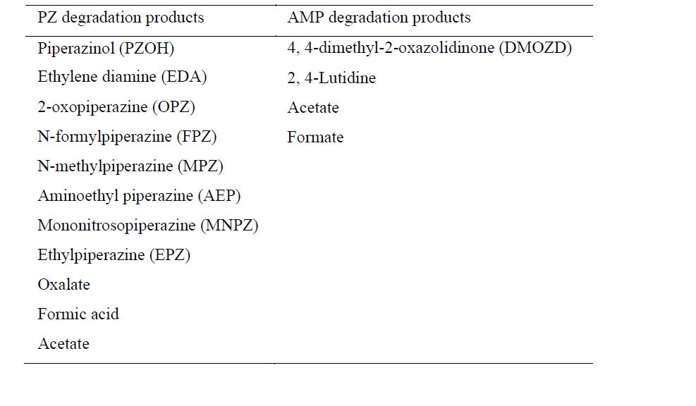
2.1 Overview of PZ Thermal Degradation
The PZ molecule has the tendency to absorb two molecules of CO2 per mole of piperazine due to the presence of two amino functional groups present in a cyclic structure. The degradation pathway of PZ solvent is not completely established for each degradation product, but the mechanism for the major degradation products of PZ have been suggested [1, 3-5]. Reactions such as bimolecular nucleophilic substitution reaction (SN2), elimination, urea generation and hydrogen-abstraction are involved in the degradation pathway [1]. Iron may also affect the formation of total formate and ammonia as both increase with increase in iron concentration, suggesting that the dissolved iron might be responsible (catalyse) for the decomposition of the intermediary oxidation products to formate and ammonia [2]. Most abundant thermal degradation products are FPZ, EDA, AEP, formate and ammonia [3]. The mechanism for the thermal degradation of PZ is shown in Fig. 1.
In the first step, PZ acts as a nucleophile at the α-carbon of another molecule of a protonated PZ (P+) in SN2 reaction to give 1-(2-aminoethyl)-ethylpiperazine (AEAEPZ) as shown in Fig. 1. AEAEPZ has the tendency to get protonated at multiple positions due to the presence of nucleophilic primary, secondary and tertiary amino functionalities (Fig. 1 to Fig. 3). In the case of protonation of the inner-secondary amine group between C4 and C5, PZ can attack at the α-carbons (C4 and C5) to yield 1- polyethylpiperazine (PEP), protonated ethylene diamine (EDA+) and two molecules of 1-(2-aminoethyl)piperazine (AEP) respectively. If the tertiary nitrogen in the AEP molecule is protonated, then the α-carbon becomes prone to an SN2 reaction with another molecule of AEP nucleophile resulting in 1,4-diaminoethylpiperazine (DAEP) and AEP+. On the other hand, AEAEPZ can react rapidly in the presence of CO2 in the solution to form internal urea. The internal urea, when protonated, can give a substitution reaction with another molecule of PZ which attacks on the C6 of this internal urea under SN2 reaction yielding other degradation products such as ammonium, CO2 and quaternary amine. Similarly, EDA can also react with CO2 to form imidazolidinone. AEP can also get protonated at multiple positions. If the protonation occurs at the terminal amine, the C7 can be approached by another molecule of AEP to yield polyAEP and ammonium while the protonation at the tertiary nitrogen gives DAEP and PZ+, as shown in Fig. 1.
PEP in its protonated form (at one of the tertiary amines in the cyclic structure) can undergo Hofmann’s elimination reaction to give 1-ethenylpiperazine and PZ. The elimination reaction is facilitated by higher temperatures and a mix of nucleophiles present in the solution. PEP can undergo Anti-Markovnikov hydration of 1-ethenylpiperazine in the presence of water to form 2-Hydroxyethylpiperazine (HEP) [1, 3-4]
If the tertiary amine of AEAEPZ gets protonated, it can react with a PZ molecule at positions C7 and C1 to yield hexamine and a molecule of AEAEPZ and PZ+ respectively (Fig.2). Similarly, protonation of the amino group in the cyclic structure of the AEAEPZ molecule followed by an attack of PZ nucleophile at C2 can give rise to the long chain hexamine shown in Fig. 3.
2.2 Overview of PZ Oxidative Degradation
The first step in the oxidative degradation pathway is the formation of peroxide radicals. The process starts with the abstraction of a proton from one of the methylene carbon in PZ molecule thus forming a free radical which can form peroxyl radical in the presence of O2. Degradation of the peroxyl radical may take place through; 1)intermolecular abstraction of proton (Fig. 4) or 2)intramolecular abstraction of proton (Fig. 5).
In the event of intermolecular abstraction of protons in an alkaline medium, peroxide (2) is generated together with •OH and •H. In the next step 2-hydroxyl-PZ (3) is formed, further oxidation results in the generation of (4). The [(2- aminoethyl) amino]acetaldehyde (5) undergoes further oxidization to give oxalic acid (7) and EDA (8). EDA can further degrade to give glycine (9) and glycolic acid (10). In a complex series of reactions oxalic acid and EDA can react to form 2-oxopiperazine (OPZ). The aldehyde (5) can also oxidize to give carboxylic acid (6) which undergoes ring closure reaction to give OPZ, as shown in (Fig. 4) [6-8].
Intramolecular proton abstraction may take place resulting in the peroxide radical which in the presence of •OH and through a homolytic cleavage of C2 ̶ C3 bond yields imine (11). Compound (11) degrades further to give unstable [(2-aminoethyl)amino}acetaldehyde] (12) and formaldehyde (13). Further degradation of (12) can form EDA (8) and formaldehyde. Formaldehyde undergoes oxidation to give formic acid (14) which in the presence of PZ can yield FPZ, see Fig. 5 [6- 8]
In other products, acetate and PZ can also react together to form acetyl piperazine (APZ), whereas, reaction of piperazine in the presence of CO2 gives piperazine carbamate, which undergoes nitrosation in the presence of nitrite to give 1-nitrosopiperazine (MNPZ), see Fig. 6 [9,10]
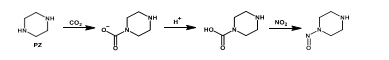
2.3 Overview of AMP Thermal Degradation
The main thermal degradation product of AMP is DMOZD. It is formed by the reaction of AMP with CO2 to form AMP-carbamate which is unstable and undergoes cyclisation and dehydration to yield the oxazolidinone DMOZD, see Fig. 7. Since AMP is branched and sterically hindered, it is less prone to further secondary degradation reactions compared with MEA. Thus, it is limiting the secondary degradation products formation. According to Gouedard et al. [11], some other thermal degradation products include 2,2-trimethylethanolamine, 4,4-trimethyloxazolidin-2-one, 4,4- dimethyl-1- hydroxytertiobutylimidazolidin-2-one, and l,3-bis(2-hydroxy-l,ldimethylethyl)urea [11,12].
![Fig. 7. AMP thermal degradation pathway through carbamate formation, followed by cyclization and dehydration to 4,4-dimethyl-1,3-oxazolidin- 2-one (DMOZD) [11].](https://gassnova.no/app/uploads/sites/5/2022/04/1-39.png)
2.4 Overview of AMP Oxidative Degradation
The mechanism for the oxidative degradation of AMP via peroxyl radical mechanism, is shown in Fig. 8. Wang et al. [7] proposed an intramolecular hydrogen abstraction from either NH or CH bond that resulted in imine and enamine formation. Both the imine and enamine can be degraded further to give (3) and (4) with the loss of OH radical. Hydrolysis of the enamine results in the formation of ammonia and formaldehyde. The hydrolysis of compound (4) can give secondary degradation products such as acetone, acetic acid ammonia, nitrate and nitrite etc. Another major product from oxidative degradation of AMP is 2,4-lutidine. The formation of lutidine goes through a series of reactions involving imine and formaldehyde, see Fig. 8 [7, 8]
![Fig. 8. AMP degradation pathway via peroxyl radical mechanisms adapted from Wang et al. [7,8]](https://gassnova.no/app/uploads/sites/5/2022/04/1-40.png)
3. CESAR1 degradation results and rates
The analysis of degradation rate is based on 2 testing campaigns performed, in 2019 ALIGN CCUS on CHP flue gas and in 2020 TCM Owners campaign on RFCC flue gas. More details for flue gas compositions can be found in [13]. Throughout the testing campaigns, samples were taken from lean amine and chemical analysis of the samples were performed to analyze the solvent composition. The main CESAR1 degradation products which were measured and quantified during testing are listed below. All measurements of degradation products were performed by Sintef.
- 2,4-lutidine
- DMOZD – 4,4-dimethyl-2-oxazolidinone
- MNPZ – N-methylpiperazine
- OPZ – 2-oxopiperazine
- Organic acids and heat stable salts
Fig. 9 demonstrates the change in degradation product concentration during the ALIGN (CHP flue gas) testing campaign. As can be seen there are 2 main zones where detailed degradation calculations and assessments have been performed.
Zone 1: Operation from September 12, 2019, to October 12, 2019, during this testing period operation the NO2 absorbed by the CESAR1 was on average 0.5 ppmv. This concentration of NO2 is considered low and was the result of constant ammonia feed to the SCR upstream of the amine plant.
Zone 2: Operation from October 12, 2019, to November 1, 2019, during this testing period operation was quite stable and the NO2 absorbed by the CESAR1 solvent was on average 2.35 ppmv. This concentration of NO2 is considered high and was the result of no ammonia feed to the SCR upstream of the amine plant. This was not a planned test, however the variation of NO2 concentration will allow a comparison of CESAR1 degradation rates with high and low NO2 concentrations.
The results clearly demonstrate an increased slope of nitrosamine formation in Zone 2, which as expected coincides with a significant increase in NO2 entering the absorber.
![Fig. 9. Degradation product concentrations in Zone 1 and Zone 2 during CESAR1 testing campaign. This figure has been presented in [14] and discussed in short.](https://gassnova.no/app/uploads/sites/5/2022/04/1-41.png)
For the 4 quantified non-volatile degradation products (DMOZD, 2,4-lutidine, MNPZ, OPZ) the total accumulation is determined for Zone 1 and Zone 2 and presented in Table 2. It should be noted that 2,4-lutidine is not included because the formation rate was observed to be zero. The rates of formation of MNPZ and OPZ have increased in Zone 2 as compared to Zone 1, due to the increased NO2 concentration. To calculate the total amine losses resulting from degradation, it is required to know the individual formation for each degradation product and to use the stoichiometric relationship with amine moles consumed. A common manner of expressing amine losses through degradation is by the following expression: Amine loss ratio = kg of amine loss/ton CO2 captured.
Table 2. Degradation products total accumulation in Zone 1 and Zone 2.
| Degradation products | Units | Zone 1 | Zone 2 |
| 4, 4-dimethyl-2-oxazolidinone (DMOZD) | kg | 38 | 19 |
| Mononitrosopiprazine (MNPZ) | kg | 40 | 158 |
| 2-oxopiperazine (OPZ) | kg | 33 | 68 |
For this calculation it is required to quantify the total amine losses through degradation and total CO2 captured in Zone 1 (low NO2) and Zone 2 (high NO2), the results are shown in Table 3. The results demonstrate that the amine loss ratio through degradation has doubled in Zone 2 as compared to Zone 1, a result of the increased NO2 concentration.
Table 3. Amine loss ratio through degradation (quantified degradation products).
| Parameter | Units | Zone 1 | Zone 2 |
| Amine loss to degradation | kg | 87 | 191 |
| CO2 captured | kg | 1971 | 2112 |
| Amine degradation loss ratio | kg/tonCO2 | 0.044 | 0.091 |
The rates of degradation above consider the quantified degradation products measured. However, it should be noted that there can be other unquantified degradation products which would contribute to additional amine loss through degradation. A way to assess if there are significant unquantified degradation products, is to observe the alkalinity or nitrogen balance for solvent samples taken during the test campaign. An assessment was done to observe how the alkalinity difference is closing for the CESAR1 solvent at different times in Zone 1 and Zone 2. This was achieved by comparing the measured solvent alkalinity versus a calculated solvent alkalinity. The measured alkalinity is based on titration results where all alkaline components (known or unknown) in the solvent will contribute to total solvent alkalinity whereas the calculated solvent alkalinity considers the solvent amines and quantified degradation products. Fig. 10 demonstrate the alkalinity difference during the testing period.
The alkalinity difference increases in Zone 2 as compared to Zone 1, where at the end of Zone 2 the alkalinity difference is around 5%. This signals that as time increases, especially with high NO2 that there are unknown or unquantified degradation products which are increasing in the CESAR1 solvent. Therefore, it can be expected that the amine loss ratios through degradation presented in Table 3 are underestimated. A revised calculation of amine loss ratio through degradation including the above alkalinity difference is shown in Table 4. The amine loss ratio in Zone 2 has increased (~ 1.85 times) from 0.091 kg amine/ton CO2 (excluding unknown degradation products) to 0.169 kg amine/ton CO2 (including estimate of unknown degradation products). There is no significant change or adjustment in Zone 1 amine loss ratio since the alkalinity difference was close to zero. Analysis performed to understand the degradation products contributing to the alkalinity difference are described in [14] and Section 6 of this article.
| Parameters | Units | Zone 1 | Zone 2 |
| Amine loss to degradation | kg | 87 | 357 |
| CO2 captured | kg | 1971 | 2112 |
| Amine degradation loss ratio | kg/tonCO2 | 0.044 | 0.17 |
A similar degradation assessment was performed for RFCC flue gas testing during the CESAR1 Owners Campaign 2 where the amine loss ratio through degradation is shown in Table 5. The results demonstrate a ~ 5 times higher amine loss ratio through degradation when the alkalinity difference calculation (0.120 kg/tonCO2) is used instead of only quantified degradation products (0.025 kg/tonCO2). It is believed that the impurities in the RFCC flue gas are contributing to additional unknown degradation products in solution, as compared to CHP flue gas testing.
Table 5. Owners 2 Campaign (RFCC) Amine loss ratio through degradation.
| Parameters | Units | Owners Campaign 2 (RFCC) |
| Amine loss to degradation (based on quantified degradation products) | kg/tonCO2 | 0.025 |
| Amine loss to degradation (based on alkalinity difference calculation) | kg/tonCO2 | 0.120 |
| CO2 captured | kg | 7,370 |
It should be noted that the amine loss ratio’s in (RFCC) are lower than the values in Table 4 (CHP). However, since the amine loss ratio is expressed as amine loss/ton of CO2 capture, the total amount of CO2 captured has a large influence. For RFCC the total CO2 captured is significantly higher than CHP due to the concentration difference in the flue gas. To illustrate this behaviour an example is presented below where key the assumptions and results are presented in Table 6. The results demonstrate the amine loss rate through degradation is ~ 2.6 times higher for RFCC flue gas (6.4 kg amine loss/hr) as compared to CHP (2.5 kg amine loss/hr) for the example below.
Table 6. Example comparing absolute amount of amine losses through degradation for CHP and RFCC flue gases.
| Parameters | Units | CHP flue gas | RFCC flue gas |
| Inlet flue gas flowrate | kmol/hr | 10,000 | 10,000 |
| Inlet CO2 concentration | vol% | 3.7 | 13.5 |
| CO2 capture percentage | % | 90 | 90 |
| Amine degradation loss ratio | kg/tonCO2 | 0.17 | 0.12 |
| CO2 captured | ton CO2/hr | 14.6 | 53.5 |
| Amine loss rate | kg/hr | 2.50 | 6.40 |
4. Degradation comparison for CESAR1 and MEA
This section will provide some comparisons between CESAR1 and MEA amine-based solvents. The MEA results on amine loss rate were extracted from a TCM publication summarizing CHP flue gas testing results in [13]. Firstly, in Table 7 the total amine loss ratio is compared, where results demonstrate significantly higher amine losses for MEA as compared for MEA, for both CHP and RFCC flue gas.
Table 7. Amine loss ratio for CESAR1 & MEA.
| Amine losses to degradation | Units | CHP flue gas | RFCC flue gas |
| CESAR1 | kg/tonCO2 | 0.171 | 0.122 |
| MEA | kg/tonCO2 | 0.6 -1.63 | 0.2-0.44 |
- Amine loss ratio calculated based on high NO2 region and alkalinity difference approach (see section 3)
- Amine loss ratio calculated based on alkalinity difference approach (see section 3)
- Total amine loss is presented for MEA. For CHP flue gas amine loss due to emission is very low (< 1%) and will not impact the comparison.
- Total amine loss is presented for MEA. For RFCC average amine loss to emission is 8% of total and will not impact the comparison.
Also, an indicator of degradation is iron (Fe) concentration in an amine solvent. As can be seen from Fig 11a below the Fe concentration is significantly lower for CESAR1 as compared to MEA, indicating lower amine degradation caused by oxidative and thermal effects.
An additional comparison of solvent degradation for CESAR1 and MEA is shown in Fig 11b. Two trends are shown, total nitrosamine (TONO) and heat stable salts (HSS) versus time. The results demonstrate that degradation to heat stable salts is significantly higher for MEA as compared to CESAR1, whereas the opposite behaviour is observed for total nitrosamines. For CESAR1, the piperazine component is a secondary amine and is very prone to nitrosamine formation in the presence of NO2. MEA on the other hand is a primary amine and forms nitrosamine at a significantly lesser rate.
5. CESAR1 thermal reclaiming
The 2020 CESAR1 TCM Owners campaigns were performed with the already used CESAR1 solvent from the ALIGN CCUS test campaign in 2019 [14]. After roughly 1600 hours of CO2 capture plant operation, reclaiming of the solvent was deemed necessary at the start of the first owners test campaign in April 2020. The main goal was to remove the solvent degradation products and metals that had accumulated during operation and refresh the solvent for the first owners test campaign. Later, after an additional 2200 hours of CO2 capture plant operation was conducted which was followed by another thermal reclamation campaign in October 2020.
Both reclaiming operation periods were conducted in a semi-continuous operation mode similarly as previously done with MEA [15]. Fig. 12 shows a process flow diagram of the TCM plant, including the reclaiming system. The reclaimer was initially filled with a mix of demineralized water and an aqueous solution of 33 wt% NaOH. The mix was heated to around 130°C in the circulation loop before the lean amine feed was started and continued at a rate of approximately 2 m3/h. Approximately 8 ml/min of NaOH was added continuously during the reclaiming. Metals, heat stable salts (HSS) and degradation products accumulated in the reclaimer while amine and water were evaporated and led back to the stripper. This operation continued for 4 days before the amine feed was stopped. A total of 4.5 times the main plant total inventory was circulated through the reclaimer during the operation period. The temperature in the reclaimer was then raised to 144 °C in between addition of water for 2 days while the remaining amine and water evaporated and the amount of waste in the reclaimer was reduced. It was suspected that the high temperature could induce further degradation in the stream going back to the stripper, although only a limited amount of solvent is exposed to this temperature. The maximum temperature for the second reclaiming was thus limited to 137 °C. The reclaimer vessel was then emptied and cleaned, and the waste sent for disposal in three intermediate bulk containers (IBCs).
Table 8 below shows the removal rates from the reclaiming operations. The solvent quality is significantly improved during this operation. The average rates of removal were highly encouraging; 94% for metals, 89% for HSS and 83% for other known degradation products and the loss of amine through waste was lower than 5%. Long boil-off time at the end of reclaiming has been beneficial in terms of low amine loss. However, caution must be taken since exposure of high temperatures during boil-off can risk further degradation. The viscosity of waste was relatively low due to the low amine concentration, which makes draining of the reclaimer waste less challenging. Precautions are needed when handling thermal reclaimer waste as the content will contain nitrosamines and other potentially harmful degradation products.
Table 8. Loss of amine and removal of degradation products, heat stable salts and metals during reclaiming of CESAR1 solvent.
| Amine loss (%) | HSS removal (%) | Metals removal (%) | Degradation products removal (%) | |
| Reclaiming April 2020 | <5 | 89 | 95 | 84 |
| Reclaiming October 2020 | <5 | 89 | 93 | 82 |
6. Way forward to gain a better knowledge on degradation
TCM has gained valuable knowledge and experience with the use of the non-proprietary solvents 30 wt% monoethanolamine (MEA) and CESAR1 for CO2 capture. TCM has a laboratory scale solvent degradation rig (SDR) to allow further investigation on solvent degradation. This SDR can mimic the process conditions and configurations designed for CO2 capture at the TCM plant. For example, similar process conditions can be in place for the flue gas, absorber and stripper as carried out during CESAR1 test campaigns [16, 17]. TCM plans to use the SDR to gain further valuable insights into the rate of solvent degradation, identification of unknown degradation products and degradation reaction mechanisms/pathways. A SDR test campaign is planned with aged CESAR1 solvent, and the results will be compared with the CESAR1 test campaigns to close the current knowledge gaps. The SDR campaign results can provide a good understanding to solvent health and environmental risks for the CESAR1 solvent systems for CO2 capture. The results can also give sufficient knowledge of the solvent degradation expected and unexpected in a real CO2 capture plant.
The basic goal of the SDR campaign will be to demonstrate the bench-scale studies of solvent process degradation to identify unknown components, which were previously difficult to analyze. Online instruments such as FTIR and Raman spectrometer will be utilized with SDR for monitoring solvent hygiene. In addition, degraded components will be qualitatively and quantitatively characterized by using an advanced liquid chromatography-mass spectroscopy (LCMS) instrument. During this study, new analysis methods will be developed for the degraded components of the LCMS instrument, this work will be carried out at TCM lab.
7. Conclusions
In this article the solvent degradation for CESAR1 has been explored. Firstly, the expected degradation mechanism’s for the main amine components (piperazine and AMP) have been presented, along with the key degradation products which have been measured and quantified during TCM testing. Results of degradation have been compiled for tests for two flues gases (1) CHP flue gas (~ 3.7 vol% CO2 and ~ 14% O2) and (2) RFCC flue gas (~ 13.5 vol% CO2 and ~ 3.2% O2). For CHP flue gas, the results indicate a strong dependency on degradation rate as the NO2 concentration entering the CO2 absorber is elevated. This increase in NO2 concentration leads to a greater amount of nitrosopiperazine and other degradation products in the solvent. As the CESAR1 solvent becomes more degraded, approximately 5% of unknown degradation products have been idenitfied. For RFCC flue gas, higher amine loss rates through degradation have been observed and it is believed this can be attributed to the increase of impurities in the RFCC flue gas as compared to the CHP flue gas. Future work at TCM is planned to identify the unknown degradation products and to determine what additional process conditions are key contributors to solvent degradation. A comparison of overall degradation rates for CESAR1 versus MEA was also presented, comparing rates of degradation under similar flue gas conditions. The results indicate significant reduction in degradation rate for CESAR1 compared to previous MEA tests performed at TCM. Lastly, thermal reclaiming experiments have been performed on the degraded CESAR1 solvent with a goal of refreshing the solvent for future tests. Two semi-continuous thermal reclaiming operations were conducted, the average rates of removal were highly encouraging; 94% for metals, 89% for HSS and 83% for other known degradation products and the loss of amine through waste was lower than 5%.
Acknowledgments
The authors gratefully acknowledge the staff of TCM DA, Gassnova, Equinor, Shell and TotalEnergies for their contribution and work at the TCM DA facility. The authors also gratefully acknowledge Gassnova, Equinor, Shell, and TotalEnergies as the owners of TCM DA for their financial support and contributions.
References
- Freeman, S.A., (PhD thesis), Thermal Degradation and Oxidation of Aqueous Piperazine. University of Texas at Austin 2011.
- S.A. Mazari et al., Degradation study of piperazine, its blends and structural analogs for CO2 capture: A review. Int. J. Greenh. Gas Control 2014, 31, 214–228.
- Nielsen, P.T., et al., Piperazine degradation in pilot plants. EnergyProc. 2013, 37, 1912–1923
- Freeman, S.A., et al. Thermal degradation of aqueous piperazine for CO2 capture. 1. Effect of process conditions and comparison of thermal stability of CO2 capture amines. Ind. Eng. Chem. Res. 2012, 51 (22), 7719–7725.
- Freeman, S. A., et al. Thermal degradation of aqueous piperazine for CO2 capture: 2. Product types and generation rates. Ind. Eng. Chem. Res. 2012,51 (22), 7726–7735.
- Namjoshi, O., et al., Thermal degradation of piperazine blends with diamines. Energy Proc. 2013, 37, 1904–1911.
- Mark J. G, et al., Kinetics of N-Nitrosopiperazine Formation from Nitrite and Piperazine in CO2 Capture. Environ. Sci. Technol.,2013, 47 (7), 3528-3534.
- Wang, T., et al., Oxidative degradation of aqueous 2-amino-2-methyl-1-propanol solvent for post combustion CO2 capture. Ind. Eng. Chem. Res. 2012, 51 (18), 6529–6536.
- Wang, T., et al., Oxidative degradation of aqueous PZ solution and AMP/PZ blends for post combustion carbon dioxide capture. Int. J. Greenh. Gas Control 2014, 24, 98–105.
- Fine, N.A., et al., Thermal decomposition of N-nitrosopiperazine. Energy Proc. 2013, 37, 1678–1686.
- Gouedard, C., et al., Amine degradation in CO2 capture. I. A review. Int. J. Greenh. Gas Control 2012 10, 244.
- Naser, S. M., et al., Thermal Degradation Rate of 2-Amino-2-methyl-1-propanol to Cyclic 4,4-Dimethyl-1,3-oxazolidin-2-one; Mechanistic Aspects and Kinetics Investigation. Ind. Eng. Chem. Res., 2017, 56, 34, 9437–9445.
- Morken., et al., CO2 capture with monoethanolamine: solvent management and environmental impacts during long term operation at the Technology Centre Mongstad. International Journal of Greenhouse Gas Control, 2019, 82, 175–183.
- Benquet, et al., First Process Results and Operational Experience with CESAR1 Solvent at TCM with High Capture Rates (ALIGN-CCUS Project). 15th International Conference on Greenhouse Gas Control Technologies, GHGT, 2021.
- Morken, et al., Degradation and Emission Results of Amine Plant Operations from MEA Testing at the CO2 Technology Centre Monstad. Energy Procedia. 2017, 114, 1245-1262.
- Aslak, E. et.al., A new test rig for studies of degradation of CO2 absorption solvents at process conditions; comparison of test rig results and pilot plant data for degradation of MEA. 2013, 37, 717-726.
- Gjernes, E. et.at., Health and environmental impact of amine based post combustion CO2 capture, Energy Procedia. 2013, 37, 2013, 735-742.
Multivariate data analysis of online-sensors and spectroscopic data for the prediction of solvent composition parameters for MEA (2022)
Lars E. Williamsa, Audun Dragesetb*, Bjørn Grungaa
aUniversity of Bergen, Department of Chemistry, Allégaten 41, 5020 Bergen, Norway bTechnology Centre Mongstad (TCM), 5954 Mongstad, Norway

Abstract

Cost-effective operation of amine-based post-combustion CO2 capture facilities is important for successfully implementing the technology on a broad industrial scale to reach current climate objectives. Technology Centre Mongstad has benchmarked performance of such technologies in a generic amine plant since 2012. This work utilized historic plant process and laboratory data collected during a test campaign with 2-aminoethan-1-ol (MEA) in 2015. The aim of this work was to employ multivariate analysis to develop models to predict laboratory results for CO2 content (Total Inorganic Carbon) and amine functionalities (total alkalinity) in the amine solvent. Predictive models were made based on process variables alone, spectroscopic data alone and data fusion models. The process model could explain 99% of the variance for total inorganic carbon in the Lean solvent stream. The Rich solvent is more chemically complex and requires the use of spectroscopic data to explain 95-99% of the variance. In this work we demonstrated how multivariate data analysis can be employed to predict solvent parameters that can be reported in real time for improved control of the capture process.
1. Introduction
Decarbonizing heavy industries is a key for achieving the carbon mitigation goals outlined in the 6th report from the Intergovernmental Panel on Climate Change (IPCC-6) [1]. Amine-based carbon capture is among the most mature technologies for decarbonizing existing industrial point sources for CO2 emissions. Technology Centre Mongstad (TCM) has operated and demonstrated generic and proprietary amine solvents for post-combustion carbon capture (PCCC) since 2012 [2]. TCM is located on the west coast of Norway in the vicinity of Equinor’s oil refinery at Mongstad. With access to two distinctly different industrial flue gases: combined-cycle gas turbine (CCGT)-based combined-heat-and-power plant (CHP) and RFCC (Residual fluid catalytic cracker) and the ability to manipulate these flue gases (through dilution and CO2 recycling), TCM can assess CO2 capture technologies under conditions that are representative of multiple industries emissions [3]. Among the main objectives of TCM’s test campaigns are risk reduction (economic and environmental) for commercial application and full-scale deployment of Carbon Capture and Storage (CCS). Key among these test campaigns are the open test campaigns with non-proprietary solvents like aqueous 2-aminoethan-1-ol (commonly known as Monoethanolamine or MEA) and the aqueous blend of 2-amino-2-methylpropan-1-ol (AMP) and Piperazine (PZ). Data and learnings from these campaigns can be disseminated in line with TCM’s purpose to ensure safe technology implementation to combat climate change.
MEA is a first-generation amine-based CO2 capture solvent. Amine based absorption is a reversible reaction between an aqueous amine and an industrial flue gas containing CO2. The basic amine functionality reacts with CO2 to form a carbamate, removing the CO2 from the gas and trapping it in the liquid phase. This reaction is carried out in the absorber containing a packed gas-liquid contactor to ensure high mass transfer between the two phases at lower temperatures (30 – 60 °C, depending on solvent and plant configuration). The reaction can then be reversed by applying heat via a steam boiler in the stripper section (see Figure 1). CO2 is released as a product gas and the liquid amine is regenerated and returned to the absorber. A capture plant operating with MEA can capture over 90% of the CO2 (advanced solvents have demonstrated over 98% capture) and generates CO2 product with high purity (99.9%) [3a]. The major challenge is the operational cost [4]. The capture plant should be operated under optimal conditions to minimize energy consumption mainly tied to removing CO2 from the solvent. This is often reported as Specific reboiler duty (SRD). To achieve this, operators are reliant on accurate gas composition data at the inlet and outlet of the absorber as well as the solvent composition. Gas composition is monitored online (via gas chromatography or infrared spectroscopy) and operators can quickly act on any changes in for example the CO2 concentration from the industrial source. In contrast, the solvent composition is usually measured through extractive samples and laboratory analysis, and results are only available after multiple hours and in some cases days.
This work utilized plant data from TCM’s MEA test campaign conducted in 2015 (July to October) funded by Gassnova, Equinor (former Statoil), Shell and Sasol (TCM’s owners in that period). The campaign’s primary objective was to conduct an updated baseline and plant performance with MEA and to verify plant mass balance over a set of operational conditions, as well as other technology knowledge gaps [5]. The plant was operated with a 30 wt% aqueous MEA solution and the CHP flue gas (3.6 vol% CO2) for most of the test period. Throughout the campaign laboratory samples were collected and analysed to (a) ensure tests were conducted with correct amine concentration, (b) record resulting lean loading (mole CO2 per mole of amine) during process optimization and (c) monitor solvent degradation and plant corrosion.
The TCM amine plant has a large array of analytical instruments in the rich (CO2 rich solvent after absorption) and lean (CO2 lean solvent after stripping solvent) streams. Among these are temperature, pH, conductivity, density, and pressure, see Figure 1. The data is used for general purpose applications in characterising the physical parameters during a test campaign. Such analytical instruments can potentially be used to predict solvent parameters currently only available via laboratory analysis like (1) Total Inorganic Carbon (TIC); a measure of CO2 in the solvent, (2) Total alkalinity (total NH functionality in the solvent as determined via an acid base titration) and (3) amine concentration. These are used to calculate the CO2 loading of the solvent (mole CO2 per mole of amine). During the campaign Total alkalinity was used as an analogue for amine concentration as the NH functionality is predominantly from MEA. It is expected that predictive models would benefit from the addition of chemical information acquired through spectroscopy, as spectroscopic methods like FTIR can give information about chemical bonds and functionality present in the solvent. Such chemical information is necessary if the degradation [6] of the solvent and its impact on the plant are to be monitored online [7].
In this paper we present how common online measurement principles like pH and conductivity can be used to predict solvent parameters which were previously only obtained through laboratory analysis. In addition, the limitations of this concept as well as how the addition of spectroscopy can improve the model accuracy is discussed. The implementation of such models can improve plant efficiency and lower the frequency of sampling and analysis resulting in a reduction of both exposure risks to operators and as well as costs for operating a laboratory.
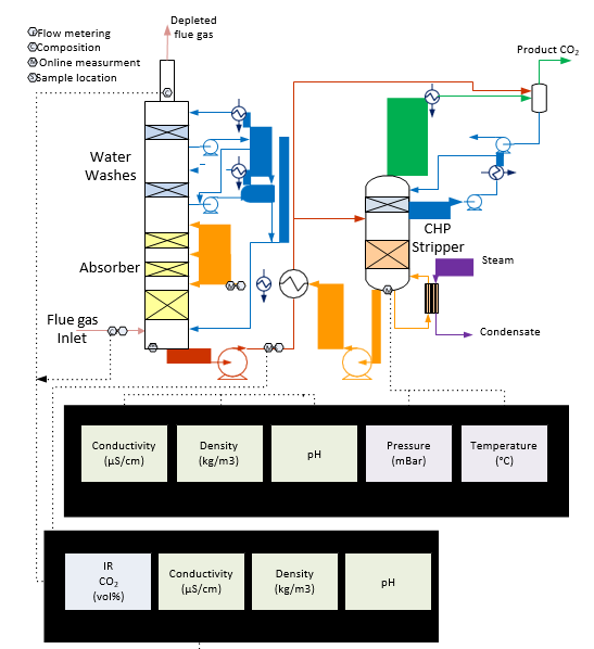
Figure 1. Simplified process flow diagram of TCM amine plant with CHP flue gas configuration. The Flue gas is introduced to the bottom of the absorber column where it is brought into contact with MEA solvent in a counter current gas absorption process in the yellow packing section. The CO2 rich solvent is sent for regeneration in the stripper where CO2 is released, the CO2 lean solvent is returned to the absorber column. Some online measurement points and variables used in this work are highlighted
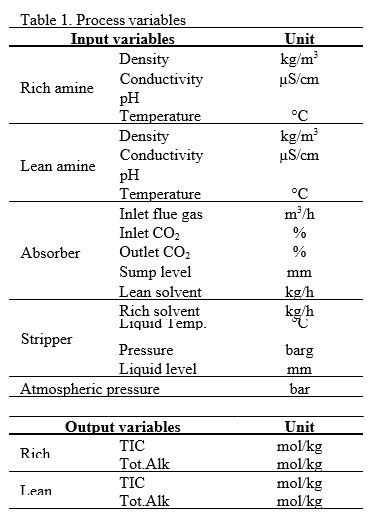
1.1 Latent variable modelling
Latent variables are linear combinations of the measured variables. They represent excellent tools for data visualization and quantitative modelling. Two main types of latent variable analysis have been used in this work. Principal Component Analysis (PCA) [8] and Partial Least Squares Regression (PLS) [9].
Any data set not based on an orthogonal design will have correlations among the variables. This makes it possible to go from a large number of measured variables to a much smaller number of latent variables while preserving the information content of the data. This concept is particularly useful for data exploration but can also be used in classification and regression analysis. In PCA, latent variables are referred to as principal components. These are constructed so that they capture as much of the variance in the data as possible. This is known as the maximum variance criterion. Each measured variable contributes to each latent variable, but the amount of contribution is different for different variables. Each measured object has a score on each latent variable, just like every object has a value for the measured variables. The collection of scores on a latent variable is referred to as a score vector, and a bivariate scatter plot of the first two score vectors after PCA is the two-dimensional plot that explains as much variation as possible. For this reason, PCA is extremely popular for data exploration, and it is used in a variety of scientific fields, although under different names.
All data contains noise. This fact means that the usefulness of principal components extends beyond data exploration. They can be used in classification and discrimination analysis, and regression. This can be done by calculating enough principal components to capture the systematic variation in the data. Using these principal components in further analysis and ignoring the residual variation left unmodelled ensures that noise in the data does not pollute the quality of the subsequent models. In this aspect, PCA can be seen as a denoising technique.
In this work, principal components have been used for data fusion [10], which is the term used for uniting different sets of data into one data set. The present work deals with traditional process data and infrared spectra used to characterize the state of an amine solution used to absorb CO2. It is tempting to combine these two measurement types to better describe the system’s state. Doing so, one immediately finds that the number of relevant spectral variables is significantly larger than the number of process variables. Simply fusing the two sets of measurements by adding one set of variables to the other will lead to a data matrix completely dominated by the spectral data. Deleting spectral variables so that the two sets become equal in size is another strategy, but there is a risk of throwing away useful information.
Furthermore, making a proper variable selection is not trivial. In this work, PCA is done on the spectral data. The number of principal components calculated and retained is enough to capture the systematic variation of the data. This number is independent of the number of variables in the data set but is decided by the number of independent sources of variation in the data. In this way one can reduce thousands of measured variables to a handful of principal components without any information loss. As the spectral variables are very correlated the reduction is substantial. This means the process data is joined with the significant score vectors from a PCA, not the measured spectral variables.
Principal components can also be used in regression analysis. This is referred to as Principal Component Regression (PCR). In multiple linear regression (MLR), one would model a response (e.g., total alkalinity of a solution) as a function of a set of measured variables, such as the process variables used in this work. There are many problems with this approach. In MLR it is assumed that the error in the independent variables is much less than the error in the response. This is not necessarily the case, and if this is violated the MLR model is not the optimal model. A further complication is that the regressors are assumed to be independent variables – they should be independent of each other. If they are not, neither the model predictions nor the interpretation of the effects of the regressors (the regression coefficients) may be trusted. Moving from a set of highly collinear measured variables to a set of orthogonal latent variables and using these as regressors elegantly avoids this problem. A further benefit of this approach is that the principal components are much less influenced by noise than the original data set. Where MLR uses all the data available, a latent variable regression model using principal components would only use the systematic part of the data as regressors.
While PCR in most cases is favourable to MLR, it is still not the preferred latent variable regression technique. The problem with the principal components is that they are constructed to capture all the main sources of systematic behaviour. Not all these systematic sources of variation will be relevant to the regression problem. A simple example would be the prediction of the concentration of a compound in a sample using spectroscopy. While changes in the analyte concentration surely impacts the spectra, so will any changes in the concentrations of other compounds present in the sample. This is systematic behaviour that will be picked up by the principal components, but it is not relevant for the prediction of our analyte. PLS is the solution to this problem.
In PLS the latent variables are calculated differently from the ones in PCA. Instead of focusing on the variance of the independent variables, PLS uses the covariance between the independent variables and the response as the latent variables. This means that the latent variables are directly related to the response modelled. Where PCR asks the question “what are the major sources of variation in my data?”, PLS asks “what part of my data varies in the same way as the response?”. This makes PLS a more powerful regression technique than PCR. They are both latent variable regression techniques, but the latent variables used in the regression are quite different.
2. Experimental section
The TCM amine plant is a generic plant designed and built by Aker Solutions and Kværner with a capacity to treat up to 60 000 Sm3/h post combustion flue gas. The plant was operated with the Combined Heat and Power flue gas with a CO2 concentration of 3.6 % and aqueous MEA (30 wt%). The absorber tower was operated with an 18- and 24- meter packing section and a lean amine flow of 43 000 – 70 000 kg/h. The stripper section was operated at 120.0 –121.5 °C. Detailed plant parameters for different test phases are described in the literature [5]. Solvent parameters were monitored via in-line liquid conductivity (Endress Hauser, resistance measurement conductivity meter), density (Coriolis mass flow, Proline Promass 80F) and pH meter (Endress Hauser, potentiometric pH measurement) installed after circulation pumps on rich and lean solvent flow (see Table 1). The process data are measured at different time intervals. In this work, values averaged over a period of 15 minutes were used for all variables.
The process data needs to be cleaned up prior to further analysis as the measurements are carried out continuously, regardless of the system state. Measurements taken during outlying conditions were removed from the data sets. Examples of outlying conditions are system shutdown periods, the recovery phase after such shutdowns and periods of MEA reclamation.
Extractive liquid samples were collected via a fast loop system equipped with a process sampler (DOPAK Inc.) by operators on a regular basis and delivered to TCM onsite laboratory for storage and further analysis.
Rich and lean liquid samples were analysed with a Bruker Alpha FTIR Spectrometer with a diamond ATR cell (Bruker Corporation). Spectra were recorded between ~4000 and ~425 cm-1. A plot of the raw spectra (Figure 2) shows that there is no relevant information above 3640 cm-1 or below 800 cm-1. The same applies to the region between 2750 cm- 1 and 1730 cm-1. These regions were removed from the spectra prior to further analysis.
The number of samples used in the models varies for the different responses and type of data. The analytical laboratory did not measure all responses for all samples, and IR spectra were not recorded for all samples. Table 2 shows the number of samples used in each model.
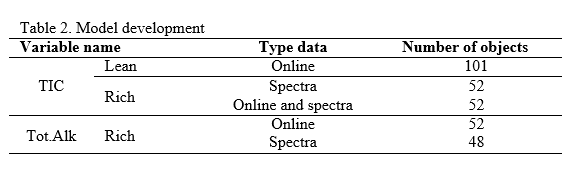
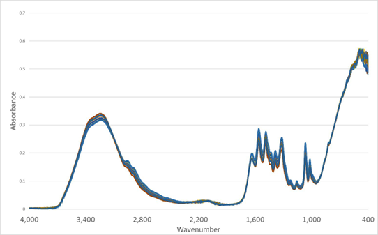
Figure 2. FTIR spectra of rich solvent samples.
Total Alkalinity is analysed via automated acid base titration with HCl (1.0 M). The reported uncertainty is 2%. Total Inorganic Carbon (TIC) is analysed with a TOC/TN Elementar (Elementar Analysensysteme GmbH). The reported uncertainty is 4%.
3. Results and discussion
3.1 Prediction of properties using only process data
3.1.1 Lean TIC predicted from process data
As the process data is a mix of variables expressed using different measurement units, the data was standardized and mean centred prior to modelling. An initial PLS regression of the process data with the lean TIC as a response yielded an 8-component model explaining more than 98 % of the variance in the TIC. The number of components was determined using cross validation [11]. This is more than satisfactory as the uncertainty in the laboratory measurements is approximately 4 %.
Not all recorded variables contribute to the regression models. Since the presence of irrelevant predictors may be of detriment to the model, care was taken to remove any predictor variables with a small regression coefficient and a large uncertainty. This also leads to a simpler model – one with fewer PLS components. The final Lean TIC model contained six PLS components and captured 99 % of the variance of the response. Figure 3 shows the regression coefficients of the variables in the final model.
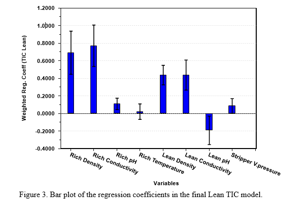
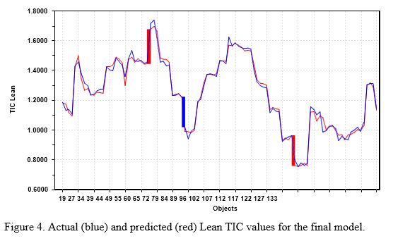
3.1.2 Rich Total alkalinity predicted from the process data
The enriched amine solution resulting from the CO2 capture is more complex chemically. Various chemical reactions take place in the mixture, and it is expected that a model based on the process data alone will struggle to explain the behaviour of the solution.
Figure 4 shows the poor performance of an optimized (irrelevant variables removed) PLS model of the Rich Total Alkalinity value. The two-component model only explains 52.81% of the response. This demonstrates that while the process variables may be enough to satisfactorily model the simpler lean system, more information is needed to obtain acceptable models for the more complex rich flow.
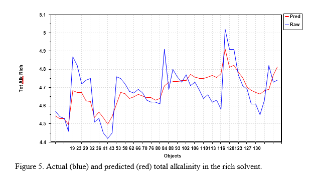
3.2 Predictions from IR spectra
As shown in 4.1.2, process data alone is not sufficient for prediction of many of the properties. Infrared spectra represent an alternative information source. An infrared spectrum contains information on the functional groups and chemical bonds present in a sample. Figure 6 shows two spectra: One from a lean sample and one from a rich sample. It is evident that the two samples have strong similarities, but also that there are differences.
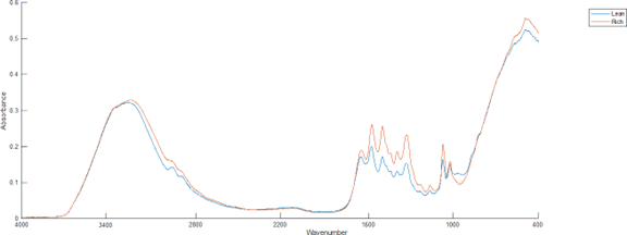
The models presented in this section use whole spectral profiles (from the regions described in the Experimental section) as predictor variables. This necessitates different pre-treatment compared to the process data. Standardization is not an appropriate tool for profile data, as that would inflate small, noisy variables and reduce the contribution from the larger, more interesting variables. The effects that usually cause problems when using spectral profiles as predictors are additive baseline effects and multiplicative effects due to light scattering. In this work, the baseline effects were handled by Savitzky-Golay second order differentiation [12] with a window size of 25 and a cubic polynomial. The multiplicative effects were handled by Extended Multiplicative Scatter Correction [13].
3.2.1 Rich Total Alkalinity modelled from IR spectra
Figure 7 shows the performance of a three component PLS model for predicting the total alkalinity in the rich samples. For this model, the Total Alkalinity values were root transformed. This improves the model quality. The model captures 95.56 % of the variance of the data and compared to the model shown in Figure 5 the IR model improves the performance to a remarkable extent.
3.2.2. Rich TIC modelled from IR spectra
Although not shown in this work, attempts were made to model the TIC of the rich solvent using only the online process data. The resulting model was only able to explain 59.46% of the response variance. It is therefore interesting to see if the performance improves when replacing the process data with the IR spectra. The best model of the IR data explained 81.66% of the response. While this is an improvement, Figure 8 shows that there is still room for improvement. The next logical thing to try is then a combination of the process and IR data.
3.3 Combining process data and IR spectra: Data fusion model of the rich TIC
An immediate challenge presents itself when trying to combine the online process data and the IR spectra. The number of spectral variables is more than 250 times larger than the process variables. This means that a simple fusion where the spectra are simply added to the process variables will lead to a data matrix completely dominated by the spectral information. More advanced fusion methods are therefore needed.
In this work, the spectral data was decomposed using Principal Component Analysis. Enough components were extracted to explain 99 % of the variance of the spectra. The number of components, which typically is quite small, was found using cross validation. The corresponding significant score vectors were subsequently appended to the process data, resulting in new variables.
Three principal components were enough to reach more than 99 % variance explained for the spectra used in the modelling of the rich TIC. The resulting model was able to explain 87 % of the variance of the response. The performance is illustrated in Figure 9. While far from perfect, it is still the best model variable, and is good enough to predict the general variations in the response.
While the model still has problems with picking up the finer changes in the response, it is clear that the combination of process and IR data has improved the performance.
4. Conclusion
This work has demonstrated the possibility of predicting relevant parameters describing the state of a MEA solvent used in CO2 capture. For some responses, solid models are achieved only using online process measurements. More complex situations benefit from the usage of IR spectra. The best models are achieved by combining both sets of data using data fusion techniques.
This work has been carried out on historical data from a campaign several years old. This represents challenges, as the detection and exclusion of outlying conditions becomes more difficult. A model is never better than the data from which it was created, so cleaning the data from outlying conditions is important.
This work demonstrates how multivariate models from process and spectral data can be used to predict the state of the solvent mixture and the efficiency of the capturing process. It is paramount that the sample set from which the model is created is representative for all the states the system may occupy in the future. Samples from both fresh and various degrees of degraded solvent states must be used. This should not represent a problem for a plant operating under relatively constant conditions.
Continuous monitoring of plant conditions is vital for cost-effective plant operation. This includes the monitoring of solvent conditions both in the lean and the rich stream. Laboratory analyses contribute to the operational expenses (OPEX) of the capture plant and a significant reduction in the scope of laboratory analysis can be a major cost saving for a full-scale plant. In addition, models can be incorporated into the control system so operators can take immediate action to keep the plant running optimally. As this work demonstrates, models can accurately predict standard laboratory parameters and can improve response time to changes in the plant. This work illustrate how technology developers can utilize process measurements and spectroscopy to improve the control of the plant. The method is not solvent or plant specific and can be used in screening historic datasets to guide further technology development.
5. Acknowledgment
The authors gratefully acknowledge the staff of TCM DA, Gassnova, Equinor, Shell and TotalEnergies for their contribution and work at the TCM DA facility. The authors also gratefully acknowledge Gassnova, Equinor, Shell, and TotalEnergies as the owners of TCM DA for their financial support and contributions.
References
[1] Intergovernmental Panel on Climate Change (IPCC), 2021: Summary for Policymakers. In: Climate Change 2021: The Physical Science Basis. Contribution of Working Group I to the Sixth Assessment Report of the Intergovernmental Panel on Climate Change [MassonDelmotte, V., P. Zhai, A. Pirani, S.L. Connors, C. Péan, S. Berger, N. Caud, Y. Chen, L. Goldfarb, M.I. Gomis, M. Huang, K. Leitzell, E. Lonnoy, J.B.R. Matthews, T.K. Maycock, T. Waterfield, O. Yelekçi, R. Yu, and B. Zhou (eds.)]. Cambridge University Press.
[2] a) E. Gjernes, S. Pedersen, D. Jain, K. I. Åsen, O. A. Hvidsten, G. de Koeijer, L. Faramarzi, T. de Cazenove, Documenting modes of operation with cost saving potential at the Technology Centre Mongstad, 14th Greenhouse Gas Control Technologies Conference Melbourne 21-26 October 2018 (GHGT-14), b) A. Morken, S. Pedersen, E. R. Kleppe, A. Wisthaler, K. Vernstad, Ø. Ullestad, N. E. Flø, L. Faramarzi, E. S. Hamborg, Energy Procedia, 114, 2017, 1245-1262, c) C. Benquet, A. Knarvik, E. Gjernes, O. A. Hvidsten, E. R. Kleppe, S. Akhter, First Process Results and Operational Experience with CESAR1 Solvent at TCM with High Capture Rates (ALIGN-CCUS Project), Proceedings of the 15th Greenhouse Gas Control Technologies Conference 15-18 March 2021.
[3] a) K. Johnsen, E. R. Kleppe, L. Faramarzi, C. Benquet, E. Gjernes, T. de Cazenove, A. K. Morken, N. Flø, M. I. Shah, M. Aronsson, Ø. Ullestad, CO2 product quality: assessment of the range and level of impurities in the CO2 product stream from MEA testing at the Technology Centre Mongstad (TCM), Proceedings of the 14th Greenhouse Gas Control Technologies Conference Melbourne 21-26 October 2018 (GHGT-14), b)G. Lombardo, M. I. Shah, B. Fostås, O. A. Hvodsten, L. Faramarzi, T. de Cazenove, H. Lepaumier, P. Rogiers, Results from testing of a Brownian diffusion filter for reducing the aerosol concentration in a residual fluidized catalytic cracker flue gas at the Technology Centre Mongstad, 14th Greenhouse Gas Control Technologies Conference Melbourne 21-26 October 2018 (GHGT-14).
[4] a) E. Gjenres, S. Pedersen, D. Jain, K. I. Åsen, O. A. Hvidsten, G, de Koijer, L. Faramerzi, T, de Cazenove, Documenting modes of operation with cost saving potential at the Technology Centre Mongstad, 14th Greenhouse Gas Control Technologies Conference Melbourne 21-26 October 2018 (GHGT-14). b) L. Faramerzi, D. Thimsen, S. Hume, A. Maxon, G. Watson, E. Gjernes, B. F. Fostås, G. Lombardo, T. Cents, A.K. Morken, M. I. Shah, T, de Cazenove, E. S. Hamborg, Results from MEA testing at the CO2 Technology Centre Mongstad: Verification of baseline results in 2015, Energy Procedia, 2017, 114, 1128-1145.
[5] E. Gjernes, S. Pedersen, T. Cents, G. Cents, G. Watson, B. F. Fostås, M. I. Shah, G. Lombardo, C. Desvingnes, N. E. Flø, A. K. Morken, T. de Cazenove, L. Faramerzi, E. S. Hamborg, Energy Procedia, 114, 2017, 1146-1157.
[6] N. E. Flø, L. Faramerzi, T. de Cazenove, O. A. Hvidsten, A. K. Morken, E. S. Hamborg, K. Vernstad, G. Watson, S. Pedersen, T. Cents, B. F. Fostås, M. I. Shah, G. Lombardo, E. Gjernes, Results from MEA Degradation and Reclaiming Processes at the CO2 Technology Centre Mongstad, Energy Procedia, 2017, 114, 1307-1324.
[7] S. Hjelmaas, E. Storheim, N. E. Flø, E. S. Thorjussen, A. K. Morken, L. Faramerzi, T. de Cazenove, E. S. Hamborg, Results from MEA amine plant corrosion processes at the CO2 Technology Centre Mongstad, Energy Procedia, 2017, 114, 1166-1178.
[8] H. Hotelling, Analysis of a complex of statistical variables into principal components, Journal of Educational. Psychology., 1933, 24, 417-441
[9] S. Wold, M. Sjöström, L. Eriksson, PLS-regression: a basic tool of chemometrics,m Chemometrics and Intelligent Laboratory Systems, 2001, 58, 109-130
[10] E. Borràs, J. Ferré, R. Boqué, M. Mestres, L. Aceña, O. Busto, Data fusion methodologies for food and beverage authentication and quality assessment – a review, Analytica Chimica Acta, 2015, 891, 1-14
[11] P. Filzmoser, B. Liebmann, K. Varmuza, Repeated double cross validation, Journal of Chemometrics, 2009, 23, 160-171
[12] A. Savitzky, M.J.E. Golay, Smoothing and Differentiation of Data by Simplified Least Squares Procedures, Analytical Chemistry, 36, 1627- 1639
[13] H. Martemns, E. Stark, Extended multiplicative signal correction and spectral interference subtraction: new preprocessing methods foir near infrared spectroscopy, Journal of Pharmaceutical and Biomedical Analysis, 1991, 9, 625-635
CO2 capture with monoethanolamine: Solvent management and environmental impacts during long term operation at the Technology Centre Mongstad (TCM) (2019)
Anne Kolstad Morkena,b,⁎, Steinar Pedersena,b, Stein Olav Nessea,b, Nina Enaasen Fløa,b, Kim Johnsena,b, Jane Karin Festea,b, Thomas de Cazenovea, Leila Faramarzia,b, Kai Vernstadc
aTechnology Centre Mongstad (TCM), 5954 Mongstad, Norway bEquinor ASA, P.O. Box 8500, 4035 Stavanger, Norway cSintef Materialer og Kjemi, Avd Bioteknologi, Sem Sælands vei 2, 7034 Trondheim, Norway

Available online 17 January 2019
1750-5836/ © 2019 Elsevier Ltd. All rights reserved.
Abstract
The owners of the Technology Centre Mongstad (TCM DA) started a monoethanolamine (MEA) test campaign in June 2017. The main objective was to produce knowledge and information that can be used to reduce the cost as well as technical, environmental and financial risks of commercial scale deployment of post-combustion capture (PCC). The campaign covered experimental activities in the amine plant from the 12th of June 2017 until the 30th of July 2018. A wide range of operating conditions were applied, thus giving a unique opportunity to study the impacts on the solvent quality, degradation behavior, corrosion tendency and emissions to the atmosphere. The current work describes how solvent quality and low emissions to atmosphere can be maintained during long- term operation by appropriate solvent management.
This article is behind a paywall. For futher information: https://www.sciencedirect.com/science/article/abs/pii/S1750583618307576?via%3Dihub
Degradation and Emission Results of Amine Plant Operations from MEA Testing at the CO2 Technology Centre Mongstad (2016)
Anne Kolstad Morkena,b,*, Steinar Pedersenb, Eirik Romslo Kleppea, Armin Wisthalerd, Kai Vernstade, Øyvind Ullestada,b, Nina Enaasen Fløa, Leila Faramarzia,b, Espen Steinseth Hamborga,b
aCO2 Technology Centre Mongstad (TCM DA), 5954 Mongstad, Norway bStatoil ASA, PO Box 8500, 4035 Stavanger, Norway cGassnova SF, Dokkvegen 10, 3920 Porsgrunn, Norway dUniversity of Oslo, Department of Chemistry, P.O. Box 1033 Blindern, 0315 Oslo, Norway eSintef Materialer og Kjemi, Avd Bioteknologi, Sem Sælands vei 2, 7034 Trondheim, Norway *Corresponding author
(http://creativecommons.org/licenses/by-nc-nd/4.0/).
Peer-review under responsibility of the organizing committee of GHGT-13.
doi: 10.1016/j.egypro.2017.03.1379
Abstract
In 2015, the CO2 Technology Centre Mongstad (TCM DA), operated a test campaign using aqueous monoethanolamine (MEA) solvent at 30 wt%. The main objective was to demonstrate and document the performance of the TCM DA Amine Plant located in Mongstad, Norway. This paper will present several aspects concerning degradation of the solvent and atmospheric emissions from amine based CO2 removal processes. The work aims to; (1) quantify the amounts and compositions of the degraded solvent (2) report results from atmospheric emissions measurements of amines and amine based degradation products; and (3) present Ambient Air measurement done during a 2 month campaign.
1. Introduction
The CO2 Technology Centre Mongstad (TCM DA) is located next to the Statoil refinery in Mongstad, Norway. TCM DA is a joint venture set up by Gassnova representing the Norwegian state, Statoil, Shell, and Sasol. The facility run by TCM DA entered the operational phase in August 2012 and it is one of the largest post-combustion CO2 capture test centres in the world. A unique aspect of the facility is that either a flue gas slipstream from a natural gas turbine based combined heat and power (CHP) plant or an equivalent volumetric flow from a residual fluidized catalytic cracker (RFCC) unit can be used for CO2 capture. The CHP flue gas contains about 3.5% CO2 and the RFCC flue gas contains about 13-14% CO2. One of the main test plants at TCM DA is a highly flexible and well-instrumented amine plant. The amine plant was designed and constructed by Aker Solutions and Kværner to accommodate a variety of technologies, with capabilities of treating flue gas streams of up to 60,000 standard cubic meters per hour. The plant is being offered to vendors of solvent based CO2 capture technologies to, among others, test; (1) the performance of their solvent technology, and (2) technologies aimed to reduce the atmospheric emissions and environmental impact of amines and amine based degradation products from such solvent based CO2 capture processes. The objective of TCM DA is to test, verify, and demonstrate CO2 capture technologies suitable for deployment at full-scale. Up to now the vendors Aker Solutions, Alstom, Cansolv Technologies Inc. and Carbon Clean Solutions Ltd. have successfully used the TCM DA facilities to verify their CO2 capture technologies.
From July to October 2015 TCM DA, in collaboration with partners, operated a test campaign using the non- proprietary aqueous monoethanolamine (MEA) solvent at 30 wt%.
2. The amine plant and operating conditions
The MEA campaign was started 6th of July 2015 with flue gas introduction to the amine plant. The campaign lasted to 17th of October 2015. Operational hours are counted as hours with both flue gas and solvent circulation. The entire campaign gave a total of 1960 hours of operation (figure 1).
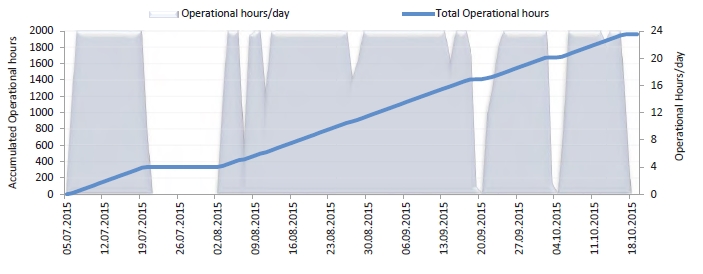
Figure 1. Overall MEA campaign operational hours, from 6th of July to 18th of October 2016.
A process flow diagram including sample points for the amine plant is given in figure 2. A more detailed description of the TCM DA amine plant and the TCM sample handling system can be found elsewhere [1,2,3]. Liquid and gas sampling, target component groups and analytical measurement techniques are described in sections 2.3 to 2.5 below.
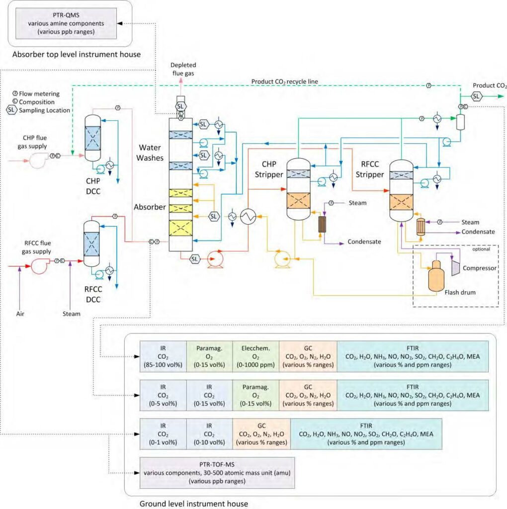
Figure 2. Process flow diagram for TCM, including online equipment’s and manual sampling locations.
Several operating conditions are important with respect to the solvent degradation and emission rates of amines and degradation products. Detailed information about the operating conditions and all the test activities and performance results from the MEA campaign, can be found in Gjernes et al [12].
The flue gas composition downstream the Direct Contact Cooler (DCC) from the CHP and the RFCC are providing a range of test conditions and the solvent will be exposed to a corresponding range in CO2 and O2 concentrations, as well as NOx, SOx and particles. Solvent amines react with the flue gas components and give rise to the degradation products as illustrated in figure 3. Degradation reactions of MEA and specific degradation products that where monitored during this campaign is given in section 3 below.
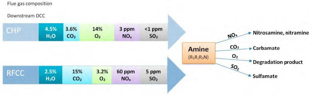
Figure 3. Typical flue gas composition influence of reaction with amines.
When the solvent is exposed to higher temperatures in combination with the flue gas components, the degradation reactions are accelerated. Also the accumulation in the solvent of transition metal elements due to corrosion may contribute to degradation [11]. Process units with high temperature exposure are the stripper and reboiler system and the hot part of the solvent circulation loop. For more process details see Table 1. The inventory and the residence time of solvent in the hot areas are decisive for degradation, for more details regarding the inventory see Flø et al [13].
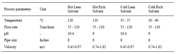
Table 1. Process parameters in the solvent circulation loop.
2.1 Liquid samples
The solvent amine, ammonia, and some degradation products were analyzed by TCM DA and Statoil Crude Oil and Products laboratories (CP Lab). Alkyl amines, aldehydes, ketone, generic nitrosamines, solvent specific nitrosamines and nitramines were analyzed by SINTEF laboratories. Total Nitrogen (Kjeldahl) was analyzed by LabNett Stjørdal, table 2 gives an overview of the different techniques used.
Organic acids and anions were measured by Ion Chromatograph (IC) and Total Heat Stable Salts (HSS) by ion exchange and following titration.
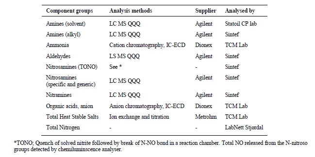
Table 2. Analytical measurements techniques.
2.2 Emission samples
TCM DA applies different measurement techniques to monitor and quantify the amounts and concentrations of emitted compounds. There are three different flue gas streams, flue gas inlet to the absorber (downstream DCC), absorber outlet and CO2-stripper outlet. Online instruments are connected via heated sampling lines to sampling probes. The amine and other emissions were monitored and confirmed by isokinetic sampling and the following online analyzers in Table 3. A full description of emission monitoring at TCM is given in Morken et al [1]. For a more detailed description of the general online equipment see Lombardo and Gjernes [6,12].
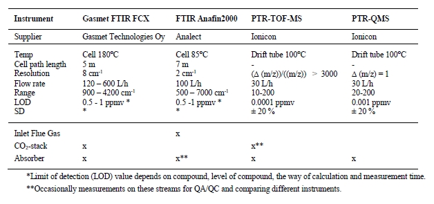
Table 3. Online instrumentation for emission monitoring at TCM.
2.3 Ambient Air measurements, instrumentation and locations
The ultra-sensitive proton-transfer-reaction quadrupole ion guide time-of-flight mass spectrometer (PTR-QiToF- MS) from IONICON was used for detecting trace gases at low pptv levels in ambient air in the vicinity of Technology Centre Mongstad. These novel ambient air measurements were performed in August and September 2015 by University of Oslo. Measurements were carried out in three different geographic locations, Sundsbø (60º46’10.1’’N, 5º09’08.6’’E), Sande (60º50’56.6’’N, 5º00’21.0’’E) and Mongstad West (60º48’45.7’’N, 5º00’43.4’’E). These sites were chosen from earlier measurement done by Norwegian Institute for Air Research (NILU) and dispersion models done by NILU [5]. For more technical details and results regarding this surveillance see Mikoviny et al [10].
3. MEA solvent and degradation theory
3.1 Oxidative and Thermal degradation
The degradation mechanisms for MEA have been extensively studied in the literature [4,5,8,11,14]. The main degradation reaction pathways with most important degradation products are indicated and proposed in figure 7 below. Oxidative degradation is induced by O2 and produces oxidized fragments of the solvent. Organic acids, ammonia and aldehydes are the main products from this degradation route. Ammonia and aldehydes are observed in the emission samples. The organic acids react with MEA and various degradation products are formed in subsequent reactions. These products are identified in the solvent samples.
The carbamate degradation route requires CO2 and fairly high temperatures. The thermal degradation of MEA occurs predominantly in the reboiler and stripper packing due to exposure to high temperature. While the initial products of thermal degradation have been identified, the kinetics of the thermal degradation pathways has not been clearly defined. Davis and Rochelle [14] indicate that thermal degradation is minor when reboiler temperature is held below 110°C but it accelerates above 130 °C. Carbamate polymerization due to high temperature is the main cause of thermal degradation of MEA. This degradation is also compounded when the CO2 loading of the solution is increased. MEA concentrations can be kept at 30 wt % to minimize thermal degradation and prevent corrosion in industrial applications.
3.2 HSS components
Heat Stable Salts (HSS) are salts in the amine solution that is not affected by heat. The heat stable salt does not regenerate in the regenerator and remains in the circulating amine system. Total HSS are measured by a titration procedure which prepares the sample with a strong cation exchange resin. Individual HSS anions are measured by Ion Chromatography (IC). The different anions measured by IC are summarized in table 4.
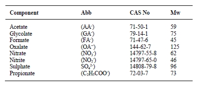
Table 4. Heat stable salts anions analyzed by TCM laboratory using Ion Chromatography.
The identified anions are summed to provide a total HSS. In general, Total HSS by titration should be the same or larger than the sum of anions by IC, figure 6 (h). Total HSS are reported as the wt% of the equivalent amount of amine. This means if HSS concentration were 1 mole/kg (eq/kg) of solution, it will be 6.1 wt% as MEA (1).

3.3 Degradation components in solvent, from emission and in Ambient Air
The degradation components measured during the MEA campaign were based on information found from literature [4]. All components from solvent and emission samples in Table 5 were analyzed by Sintef. The analyzing measuring technique was primarily LC-MS-QQQ. The mixture of the different degradation components are hereafter called D-mix. Analysis of Ambient Air components were done by University of Oslo [10].
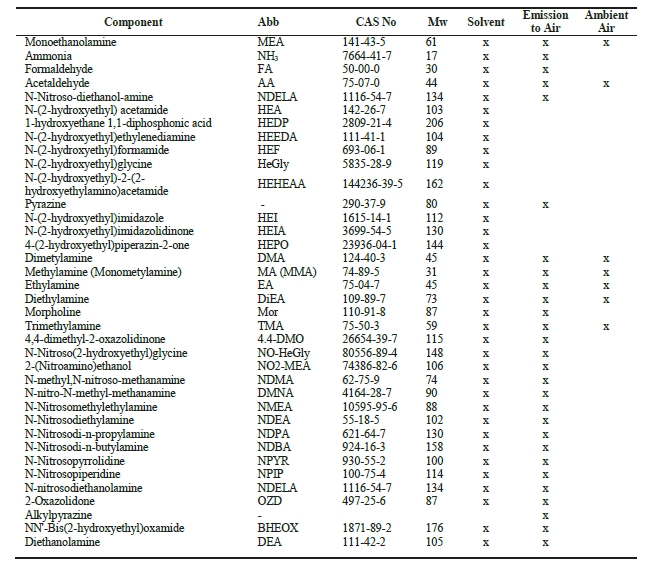
Table 5. Degradation products and measurements in solvent, emission from amine plant absorber stack and in Ambient Air.
4. Results and discussions
The first observable sign of degradation was color change of the solvent. The color of the solvent changed rapidly after the first contact with the flue gas. Samples taken before introduction of flue gas show a colorless solvent. Only hours after start up, the color started to change from colorless to yellow, and more and more orange and dark brown as seen in figure 4. After reclaiming 12th of October, the color is more like the color that appeared in the start of the campaign when the solvent was fresh.
Figure 4. Pictures of samples taken during the campaign. The color change gives an indication on how degraded the solvent is. The samples are from left to right after: 0, 1300, 1830, 1870 and 1920 hours of operation.
4.1 Heat stable salts in the solvent
Figure 5 and 6 shows how the levels of organic acids and anions developed during the entire campaign. Figure 5 shows overall heat stable salts development where 5a) are Total Heat Stable salts reported as wt% MEA, and 5b) results from individually IC results from each component. Figure 6 (a-g) shows more detailed development of all the individual components. The main anion formed is formate and the level of this component reach 3000 mg/L before reclaiming. Glyoxylic acid is assumed to be one of the formed organic acids during the degradation process [7]. It was not possible to analyze for this component as there were no available method at the time. An unknown component of significant response on the IC chromatogram was found. The area of the unknown component in the chromatogram was significant, and the component was calibrated with a mix of the other components. The result from this unknown component is rather uncertain, see figure 6 g). All other IC results have a repeatability uncertainty of ± 20%.
Figure 5. (a) Total Heat stable salt concentration; (b) Results from Anion IC analysis.
Figure 6. (a) Formate concentration, mg/L; (b) Glycolate concentration, mg/L; (c) Acetate concentration, mg/L; (d) Nitrate concentration, mg/L; (e) Oxalate concentration, mg/L; (f) Sulphate concentration, mg/L (g) unknown component, mg/L; (h) Total HSS and sum anions presented as mole/kg.
Propionate (C2H5COO–) and nitrite (NO2-) were not detected above 10 mg/L which is the limit of detection on the Ion Chromatograph.
4.2 Degradation products in the solvent
A simplified scheme for MEA degradation is proposed in figure 7. Oxidation reactions lead to formation of the organic acids and the emission products ammonia and aldehydes. This is indicated in the left blue square of the figure. Reactions between MEA and the organic acids, CO2 and additional free MEA lead to formation of the degradation products identified in the lean solvent samples. This is indicated in the large red square of the figure. A nitrogen mass balance based on solvent analysis are presented and compared to literature data in section 4.5 below.
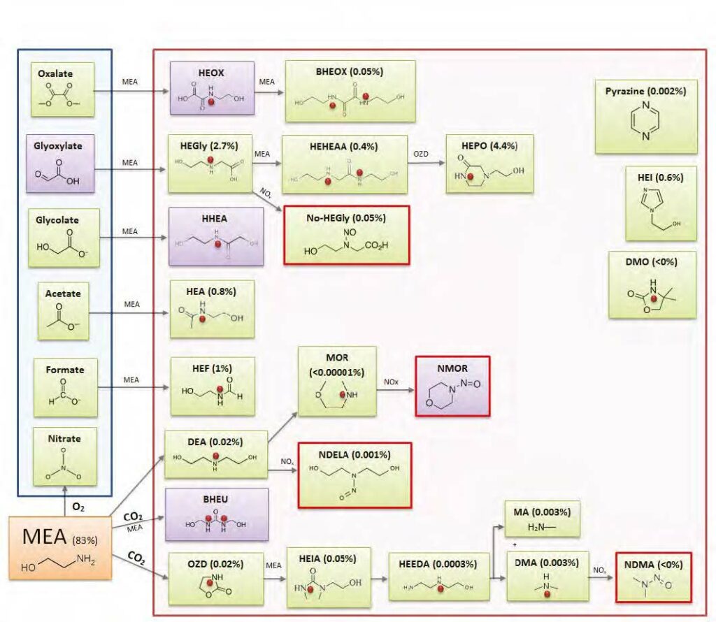
Figure 7. Proposed overall degradation scheme for monoethanolamine. Scheme is simplified and intermediate amine compounds may form.

The rate of formation of the degradation products is a function of temperature (faster kinetics), CO2 loading (more carbamate present), and MEA concentration. The identified degradation products in the solvent samples and the accumulation of these as function of operational hours are shown in figure 8.TCM performed a MIST test after 1314 hours of operation and also did a CO2 recycling test with higher CO2 content in the CHP flue gas [12]. The results shown after 1314 hours are not consistent with the other samples and cannot be explained. Results from the reclaiming part of the 2015 MEA campaign is given in [13].
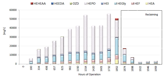
Figure 8. Main degradation products during the entire campaign. The component names and abbreviation is given in table 5 above.
It is seen that the dominant degradation products in the solvent are N-(2-hydroxyethyl)glycine (HeGly) and 4-(2- hydroxyethyl)piperazine-2-one (HEPO). This corresponds to the oxidation pathway via glyoxylate and subsequent reaction with MEA given in figure 7. The identification of the nitroso-compound nitroso-Hegly (No-HeGly) in the solvent further confirms this degradation route.
4.3 Nitroso- and Nitramines in solvent
Two solvent specific nitrosamines, N-nitrosodiethanolamine (NDELA) and N-nitroso-2-hydroxyethyl-glycine (Nitroso-HeGly), were detected in the solvent as the degradation process progressed. The total concentrations of nitrosamines (TONO) were measured to be 2351 µmol/L after 1850 hours of operation, see figure 9. Since MEA is a primary amine it is not expected to form a stable nitrosamine. The identified compounds are thus formed from secondary amines occurring as impurities in the solvent or being formed during the degradation reactions. As is shown in Figure 9 a), there are still some unidentified nitrosamines in the degraded solvent sample. These nitrosamines are formed from high molecular weight amines and have low volatility. Figure 9 b) shows a decrease in the level of total nitrosamines after reclaiming of the solvent.
Nitrosamines are formed after reaction with NOx in the flue gas [8]. During the MIST test, RFCC flue gas was used, and as this flue gas contains more NOx than flue gas from the Combined Heat and Power Plant, this could explain the higher amount of nitrosamines in this MEA2 campaign compared with the first MEA1 campaign from TCM [1].
The solvent specific nitramine (MEA-NO2) was detected at a concentration of approximately 4 mg/L after 1850 hours of operation. Methylnitramine (MA-NO2) and Dimethylnitramine (DMA-NO2) were also analyzed, but the responses on the LC MS QQQ were below the limit of detection (< 0.1 mg/L).
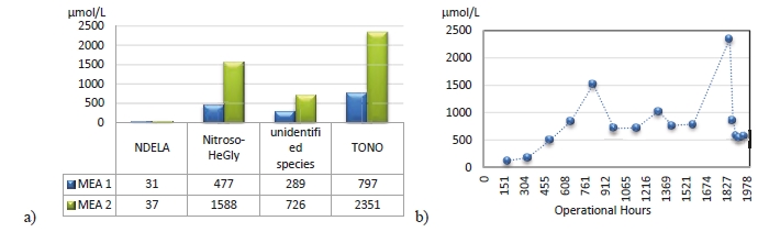
Figure 9. a) Nitrosamines in Lean MEA after 1850 operational hours. Results from the first MEA campaign (MEA 1) and this campaign (MEA 2) b) TONO measurements through the entire campaign.
4.4 Nitrogen mass balance of the solvent
A nitrogen balance of the solvent was done after 1850 hours of operation, just before reclaiming, see table 6.
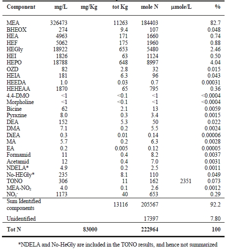
Table 6. A nitrogen mass balance of the solvent was done after 1850 operational hours.
Total Nitrogen in lean amine was measured to be 8.3 wt%, which give a total of 222964 mole N. The sum of the different degradation products found gives a total of 205567 moles. This gives 7.8 mole% of nitrogen that is not found by analysis, these components are hereafter called unidentified components. Some of the unidentified components are assumed to be long chain molecules. Dissolved ammonium and ammonia in the solvent were not measured; this means that they will presumably have some contribution to the amount of the unidentified components. Table 6 shows an overview of all the components that were analyzed, and the contributions of each component to the total amount of nitrogen.
4.5 Solvent loss
Excluding plant leakage, MEA loss can occur in the following ways:
- MEA emitted via Absorber (after water wash section)
- MEA emitted via stripper upper product after the condenser
- MEA degraded product via NH3 formation, which is detected after the wash section and from the CO2 product stream
- Liquid sampling, which was taken for analysis
- Unexpected loss due to leakage through joints and pumps
- Wash water (absorber, stripper)
- Reclaimer waste
Lab samples and reclaimer waste are a part of the total inventory calculation. MEA was charged into the amine makeup tank from trucks. From the amine make up tank, MEA can either be charged into the storage tank or directly to the process loop. A total of 30088 Kg of pure MEA was filled into the makeup tank, while a total of 23208 Kg of MEA was discharged from the plant after the end of campaign. This gave a total loss of 7622 Kg pure MEA. Total CO2 capture in the campaign was 4941 ton, and this give a loss of 1.5 kg MEA/ton CO2 captured.
A nitrogen mass balance of the total solvent system was also done. The accumulated NH3 emission from the absorber and stripper corresponds to approximately 67% of the total MEA loss, while the nitrogen detected identified degradation compounds (D-mix) constitutes approximately 16% of the MEA loss. Table 7 gives a short summary of the degraded product produced per mole amine lost. These results are similar to the results reported by IEAGHG [11]. Total Nitrogen analysis was performed, and it is reasonable to assume that long-chain degradation compounds constitute some amount of the unidentified loss.
The nitrogen mass balance for the entire campaign gives a loss of MEA that corresponds to 1.6 kg MEA/ton CO2 captured. There is a small gap between the two different methods of calculation, and average value is used. From this MEA 2 campaign it is concluded that the loss of solvent was 1.6 ± 0.1 kg/ton CO2 captured.
5. Emissions of amines and amine based degradation products
5.1 Analysis of emission from depleted flue gas
Emission to Air from TCM DA amine plant has two sources, the amine absorber and the CO2-stack. At TCM the CO2 product stream is sent into the atmosphere, which will not be the case for a full-scale CO2 capture plant. As the contribution from this stream is small considered to the absorber (1-3%), data from this stream is not given in this paper.
TCM DA applies different measurement techniques to monitor and quantify the amounts and concentrations of emitted compounds. A description of the TCM DA overall system for emission control and monitoring is given elsewhere [1]. The emission was followed up by FTIR, PTR-TOF-MS, PTR-QMS, isokinetic sampling and by 3rd party (FORCE Technology) [9].
MEA emissions are highly related to aerosols in the flue gas [6]. Even at low mass concentrations of aerosols, increased MEA emissions have been measured and reported. In September 2015 TCM investigated the relation between flue gas particle content, mainly related to sulphuric acid mist particles and dust, and corresponding MEA amine emissions. This “MIST test” was based on aerosol number concentration and size distribution, to evaluate the maximum aerosol number concentration acceptable for operation with a solvent based on MEA [6]. TCM received a temporary emission permit given for this campaign from the Norwegian environmental agency (NEA). The temporary permit gave allowance to increase MEA emission from 6 ppmV to 500 ppmV for maximum 4 days of testing.
The Mist test was a planned temporary campaign lasting for only two weeks. The rest of the MEA campaign were performed without issues regarding mist, impurities and aerosols, as flue gas from the combined heat and power plant does not contain particles and impurities. Detailed information about all the test activities and performance from the MEA campaign can be found in Gjernes et al [12].
Figures 10 – 13 provide the daily average ammonia, MEA, acetaldehyde and formaldehyde emissions and operational hours throughout the campaign. Some daily averages of ammonia emissions indicate higher emissions than allowed in the TCM DA emission permit. Any such emission peaks were communicated to the NEA. These incidents were administratively handled by NEA, and the campaign continued as planned. These higher levels were due to amine plant start-up activities, where molecular ammonia (or other amine compounds), i.e. ammonia (or other amine compounds) are unreacted with CO2, are by convection transferred by the flue gas through the absorber and eventually emitted to atmosphere. The emissions follow a Gaussian like trend, i.e. an emission peak is observed until the emission levels settles at a lower steady state level. Test activities with increased CO2 content in the flue gas combined with high temperatures in the solvent, water washes and flue gas, gave high ammonia emissions.
A start-up procedure conducted in the following order will reduce such start-up emission peaks;
- MEA solvent circulation starts at ambient temperatures
- Flue gas is introduced and the CO2 loading process of the entire MEA solvent inventory occurs at ambient temperatures, until CO2 in the MEA solvent are in equilibrium with CO2 in the incoming flue gas

- Heat is applied to the stripper section in order start the continuous CO2 removal process
By following the aforementioned start-up order, the amount of emitted molecular ammonia and amine compounds are decreased as the presence of these compounds in the gas phase inside the absorber is reduced, and hence less gaseous ammonia and amine compounds are transferred through the absorber by convection. 19th of May 2016, TCM received a new permanent emission permit from NEA allowing 100 ppmV ammonia emissions as a daily average.
Figure 10. Daily average Ammonia (NH3) ppmV emission from absorber measured by online FTIR, PTR-TOF-MS and isokinetic sampling, (isokinetic sampling is for a 2 hour period).
Figure 11. Daily average Monoethanolamine (MEA) ppmV emission from absorber measured by online FTIR, PTR-TOF-MS and isokinetic sampling, (isokinetic sampling is for a 2 hour period).
Figure 12. Daily average Acetaldehyde ppmV emission from absorber measured by online FTIR and PTR-TOF-MS.
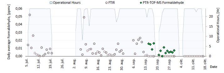
Figure 13. Daily average Formaldehyde ppmV emission from absorber measured by online FTIR and PTR-TOF-MS.
For achieving the TCM objectives, it is important that variables are measured with high degree of accuracy. This will ensure that high quality data are obtained and thus a high quality of test results can be provided. This is significant not only for technology test reports but also for emissions reporting to the Norwegian Environmental Agency (NEA). A failure to estimate the inaccuracies of measurements will complicate the test planning, reporting to NEA and operation and maintenance of the test facility. Apart from accuracies of different variables, repeatability or precision of measurements for each of the variables on different streams also needs to be estimated. One quality assurance (QA) test is to compare different monitoring techniques. This was done during the MIST test, and depleted flue gas out of the absorber was measured by four different independent measurements; two FTIR’s, PTR- TOF-MS and PTR-QMS. All the different measurement techniques showed very similar results. The result of this QA is shown in figure 14 and 15. TCM is a demo-plant where many types of online emission measurement equipment are tested, providing useful information for commercial projects.
Seven emission isokinetic sampling campaigns have been carried out in order to follow up on emissions form the absorber. Results from these measurements can be found in table 8. Overall the results are similar to the results reported by Morken et al [1].
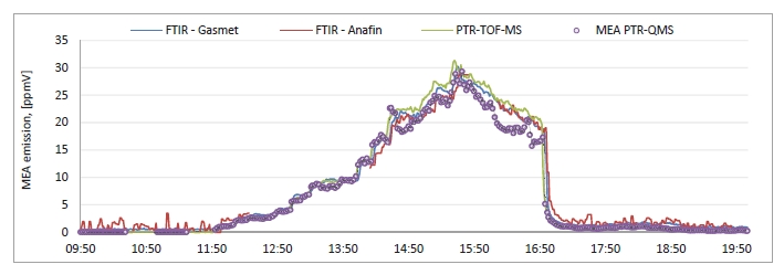
Figure 14. Simultaneously online measurement of MEA emission from amine absorber 16th of September 2015. The online equipment’s are two independent FTIR’s, PTR-TOF-MS and PTR-QMS.
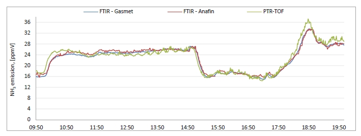
Figure 15. Simultaneously online measurement of ammonia (NH3) emission from amine absorber 16th of September 2015. The online equipment’s are two independent FTIR’s and PTR-TOF-MS.
TCM has shown earlier that the absorber wash water sections are found to effectively reduce possible atmospheric emissions from amine based solvent system [1]. Atmospheric emissions of monoethanolamine (MEA) were very low throughout the entire campaign, and determined to be in the parts per billion (ppb) ranges.
Atmospheric emissions of MEA amine based degradation products such as nitrosamines and nitramines were below detectable levels. Atmospheric emissions of alkyl amines in the low ppb range. Results from isokinetic measurements can be seen in table 8. These results confirm the emission results from earlier MEA campaign at TCM [1].
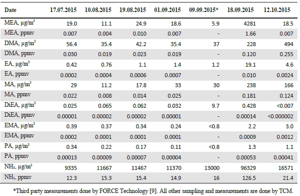
Table 8. Result from isokinetic gas emission measurements from the entire MEA campaign.
Conclusions
During the MEA 2015 campaign at TCM the degradation products being formed in the solvent and released to the atmosphere were closely monitored. Based on an overall nitrogen mass balance it was concluded that less than 8% of total nitrogen introduced into the plant was not identified. The solvent loss calculated as pure MEA was 1.6 ±
0.1 kg/ton CO2 captured. The major contributors to the loss were ammonia emission (67% of loss) and identified degradation products in the solvent (16% of loss). Emissions to air from the absorber stack were monitored by five different independent on-line measurement instruments and by regular manual sampling. The four on-line methods provided very similar results. The manual sampling results confirmed results from earlier MEA campaign at TCM. The MEA and alkyl amines emissions are in the parts per billion ranges and nitrosamines and nitramines were below detectable levels.
Acknowledgements
The authors gratefully acknowledge the staff of TCM DA, Gassnova, Statoil, Shell and Sasol for their contribution and work at the TCM DA facility. The authors also gratefully acknowledge The TCM DA operation team, lab team at TCM DA and Statoil CP laboratory, Technology Committee, University of Oslo and Sintef for their contribution and work at the TCM DA facilities.
References
- Morken AK, Nenseter B, Pedersen S, Chhaganlal M, Feste J, Tyborgnes RB, Ullestad Ø, Ulvatn H, Zhu L, Mikoviny T, Wisthaler A, Cents T, Bade OM, Knudsen J, De Koeijer G, Falk-Pedersen O, Hamborg ES. Emission results of amine plant operations from MEA testing at the CO2 Technology Centre Mongstad, Energy Procedia 63, 6023-6038.
- Thimsen D, Maxson A, Smith V, Cents T, Falk-Pedersen O, Gorset O, Hamborg E S. Results from MEA testing at the CO2 Technology Centre Mongstad. Part I: Post-Combustion CO2 Capture Testing Methodology. Energy Procedia 2014.
- Hamborg ES, Smith V, Cents T, Brigman N, Falk-Pedersen O, Chhaganlal M, Feste J K, Ullestad Ø, Ulvatn H, Gorset O, Askestad I, Gram L K, Fostås B F, Shah M I, Maxson A, Thimsen D. Results from MEA testing at the CO2 Technology Centre Mongstad. Part II: Verification of baseline results. Energy Procedia 2014
- Da Silva EF, Hoff KA, Booth A; Emissions from CO2 capture plants; an overview, Energy Procedia 37 (2013) 784-790
- Lepaumier H, Picq D, Carrette P-L, New Amines for CO2 Capture. I. Mechanisms of Amine Degradation in the Presence of CO2, Ind. Eng. Chem. Res., 2009, 48 (20), pp 9061–9067
- Lombardo G, Fostås BF, Shah MI, Morken AK, Hvidsten OA, Mertens J, Hamborg ES. Results from aerosol measurement in amine plant treating gas turbine and residue catalytic cracker flue gases at the CO2 Technology Centre Mongstad. Energy Procedia (GHGT-13), Forthcoming 2017.
- Vevelstad SJ, Eide-Haugmo I, Da Silva EF, Svendsen HF, Degradation of MEA; a theoretical study, Energy Procedia 4 (2011) 1608–1615
- Fostås B, Gangstad A, Nenseter B, Pedersen S, Sjøvoll M, Sørensen AL, Effects of NOx in the flue gas degradation of MEA, Energy Procedia 4 (2011) 1566–1573
- Faramarzi L, Thimsen D, Hume S, Maxson A, Watson G, Pedersen S, Gjernes E, Fostås BF, Lombardo G, Cents T, Morken AK, Shah MI, de Cazenove T, Hamborg ES. Results from MEA testing at the CO2 Technology Centre Mongstad: Verification of baseline results in 2015. Energy Procedia (GHGT-13), Forthcoming 2017.
- Mikoviny T, Nielsen C.J, Tana W, Wisthaler A , Zhu L, Morken A.K, Nilsen T.N, Ambient Measurements of Amines by PTR-QiTOF: Instrument Performance Assessment and Results from Field Measurements in the Vicinity of TCM, Mongstad, Forthcoming 2017.
- IEAGHG “Evaluation of reclaimer sludge disposal from post-combustion CO2 capture”, 2015/02, March 2014
- Gjernes E, Pedersen S, Cents T, Watson G, Fostås BF, Shah MI, Lombardo G, Desvignes C, Flø NE, Morken AK, de Cazenove T, Faramarzi L, Hamborg ES. Results from 30 wt% MEA performance testing at the CO2 Technology Centre Mongstad. Energy Procedia (GHGT-13), Forthcoming 2017.
- Flø NE, Faramarzi L, de Cazenove T, Hvidtsten OA, Morken AK, Hamborg ES, Vernstad K, Watson G, Pedersen S, Cents T, Fostås BF, Shah MI, Lombardo G, Gjernes E. Results from MEA degradation and reclaiming processes at the CO2 Technology Centre Mongstad. Energy Procedia (GHGT-13), Forthcoming 2017.
- Davis J, Rochelle G, Thermal degradation of monoethanolamine at stripper conditions, Energy Procedia 1 (2009) 327-333.
Results from MEA Degradation and Reclaiming Processes at the CO2 Technology Centre Mongstad (2016))
Nina Enaasen Fløa, Leila Faramarzia,b, Thomas de Cazenovea, Odd Arne Hvidstena,b, Anne Kolstad Morkena,b, Espen Steinseth Hamborga,b,*, Kai Vernstadc, Guillaume Watsond, Steinar Pedersenb, Toine Centse, Berit F. Foståsb, Muhammad Ismail Shaha,f, Gerard Lombardoa,f, Erik Gjernesf
aCO2 Technology Centre Mongstad, 5954 Mongstad, Norway bStatoil ASA, PO Box 8500, 4035 Stavanger, Norway cSINTEF, Strindveien 4, 7034 Trondheim, Norway dShell Global Solutions International B.V., PO Box 663, 2501CR The Hague, The Netherlands eSasol Technology, PO Box 5486, Johannesburg 2000, South Africa fGassnova SF, Dokkvegen 10, 3920 Porsgrunn, Norway *Corresponding author
(http://creativecommons.org/licenses/by-nc-nd/4.0/).
Peer-review under responsibility of the organizing committee of GHGT-13.
doi: 10.1016/j.egypro.2017.03.1899
Abstract
In 2015, the CO2 Technology Center Mongstad (TCM DA), operated a test campaign using aqueous monoethanolamine (MEA) solvent at 30 wt%. The main objective was to demonstrate and document the performance of the TCM DA Amine Plant located in Mongstad, Norway. As part of the test campaign, thermal reclaiming was performed in order to eliminate accumulated degradation products and improve the solvent performance. This paper presents results and discussions concerning formation and monitoring of amine degradation products along with experiences related to the thermal reclaiming process and its operational procedure. Evaluations of the efficiency of thermal reclaiming and the solvent improvement after reclaiming are also presented.
1. Introduction
The CO2 Technology Centre Mongstad (TCM DA) is located next to the Statoil refinery in Mongstad, Norway. TCM DA is a joint venture set up by Gassnova representing the Norwegian state, Statoil, Shell, and Sasol. The facility run by TCM DA entered the operational phase in August 2012 and it is one of the largest post-combustion CO2 capture test centres in the world. A unique aspect of the facility is that either a flue gas slipstream from a natural gas turbine based combined heat and power (CHP) plant or an equivalent volumetric flow from a residual fluidized catalytic cracker (RFCC) unit can be used for CO2 capture. The CHP flue gas contains about 3.5% CO2 and the RFCC flue gas contains about 13-14% CO2. One of the main test plants at TCM DA is a highly flexible and well-instrumented amine plant. The amine plant was designed and constructed by Aker Solutions and Kværner to accommodate a variety of technologies, with capabilities of treating flue gas streams of up to 60,000 standard cubic meters per hour. The plant is being offered to vendors of solvent based CO2 capture technologies to, among others, test; (1) the performance of their solvent technology, and (2) technologies aimed to reduce the atmospheric emissions and environmental impact of amines and amine based degradation products from such solvent based CO2 capture processes. The objective of TCM DA is to test, verify, and demonstrate CO2 capture technologies suitable for deployment at full-scale. Up to now the vendors Aker Solutions, Alstom, Shell Cansolv Technologies Inc. and Carbon Clean Solutions Ltd. have successfully used the TCM DA facilities to verify their CO2 capture technologies. From July to October 2015 TCM DA, in collaboration with partners, operated a test campaign using the non- proprietary aqueous monoethanolamine (MEA) solvent at 30 wt%. After testing a variety of process conditions for a total of 1843 hours, clear evidence of solvent degradation was observed. The test campaign proceeded with thermal reclaiming of the solvent in order to eliminate accumulated degradation products and demonstrate improvement of solvent performance. This work presents results concerning MEA degradation monitoring and reclaiming operation at TCM DA. Various design and operational factors that affect degradation rates are discussed, the efficiency of thermal reclaiming is estimated and experiences related to the reclaiming process and its operational procedure is shared.
1.1 Solvent degradation mechanisms
Amine solvents degrade due to exposure to heat (thermal degradation), presence of oxygen (oxidative degradation) and reactions of the amine with flue gas contaminants such as SOx, NOx, halogenated compounds, hydrocarbons and other impurities. Thermal degradation occurs mainly in the stripper section and is strongly dependent on the stripper operating temperature. The main thermal degradation products in MEA are Oxazolidin-2- one (OZD), MEA urea, HEIA, HEEDA [1]. The rate of formation of these products depend on the operating temperature (faster kinetics), CO2 loading (more carbamate present) and MEA concentration. Oxidative degradation is mainly an issue for post-combustion CO2 capture where the solvent is exposed to oxygen present in the flue gas. This occurs mainly in the absorber, where the level of oxygen is significant. Amine oxidation is also shown to be catalyzed by transition metal ions and will typically results in formation of ammonia and different organic acids [2]. In a second step, the organic acids will form heat stable salts (HSS) which are difficult to regenerate under normal regeneration conditions (atmospheric pressure and temperature around 120°C) [1]. These salts will therefore remain and accumulate in the circulated solvent. Amine degradation may also be induced by flue gas contaminants such as sulfur, polysulfide and CO. This issue has become especially evident for oil refinery flue gases such as gas originating from RFCC units [2]. Nonvolatile contaminants causing amine degradation can also arise from other sources such as make-up water, anti-foam agents, lubricants and corrosion inhibitors [2].
Several degradation processes often occur simultaneously to produce a wide range of degradation products. Accumulation of amine degradation products affects the solvent properties. They are known to increase the solvent viscosity and surface tension which again affects heat transfer coefficients, diffusion coefficients, and mass transfer rates [3]. This will again lead to loss of solvent capacity and increased energy numbers. Further, degradation products might lead to corrosion, fouling and foaming [2], which again increases operational and maintenance costs and might cause long-term technical integrity issues. Dissolved metal elements originating from corrosion are also as mentioned above expected to contribute as catalysts for oxidative degradation [1].
1.2 Solvent refreshing options
In order to reduce the impact of unwanted impurities and minimize the operational and maintenance issues listed above, a number of techniques have been suggested. Wang et al. (2015) have published an extensive review of amine reclaiming technologies and other techniques to handle this issue, including purging (bleed and feed), neutralization, ion exchange, adsorption, electrodialysis, and different thermal reclamation techniques [4]. Dumée et al. (2012) also presents a thorough comparison of the most promising techniques [1]. A summary is provided below.
- Bleed and feed
Bleed and feed is a simple operational procedure where a portion of the degraded solvent is continuously or periodically purged and replaced with fresh solvent. However, amine replacement and disposal might make this technique rather costly, particularly for specialized and expensive solvents. Further, a certain level of degradation products needs to build up before effecting bleed and feed in order to minimize replacement and disposal costs.
- Neutralization
Neutralization converts amine HSS to sodium or potassium HSS by addition of NaOH or KOH, according to the following reaction using NaOH as an example:
NaOH + [AmineH+ RCOO– ] ➔ Amine + H 0 + [Na+ RCOO– ] (1)
Neutralization maintains the amine capacity; however, there is no reduction in salt content of the solvent. The amine becomes more and more contaminated by salts that contribute to higher solvent density and viscosity, reduced surface tension, and possibly foaming and fouling. Eventually, the solvent needs to be discarded.
- Ion exchange
Ion exchange is a technology where the amine HSS ion is replaced with a friendlier ion. For example, an anion exchange removes HSS anions, replacing them with hydroxide ions, which frees the amine and let it return together with water to the process. The HSS anions are later removed from the resin by regeneration with NaOH. The practice of removing HSS from amine systems by ion exchange has presented many technical and operational challenges, and several researchers report doubt in the practical efficiency for amine applications. High consumption of chemical and water for resin regeneration together with generation of large amounts of waste are mentioned as other disadvantages. Further, ion exchangers are not capable of removing uncharged contaminants, i.e. degradation products originating from thermal degradation. It is still regarded a relatively economical method, especially for low levels of contaminants. However, if poorly designed and/or operated it can cause significant solvent losses and sodium slippage into the main amine process.
- Adsorption
Adsorption on activated carbon is a widely used method to remove high-boiling or surface active organic compounds [5]. However, activated carbon it is not able to remove significant amount of degradation products [2].
- Electrodialysis
Electrodialysis has also been suggested as a method to purify amine solutions. It uses a stack of alternating anionic and cationic ion-exchange membranes to selectively remove charged contaminants from the solvent [1]. The main disadvantage also for this method is inability to remove uncharged amine degradation products originating from thermal degradation and hydrocarbons [2].
- Thermal reclaiming
Thermal reclaiming is usually conducted on a small slipstream extracted from the stripper reboiler on a semi- continuous basis [2, 5]. The amine solution is vaporized in the reclaimer vessel and returned as vapour to the main process, while the less volatile degradation products and other contaminants accumulate in the reclaimer vessel bottoms. Stoichiometric addition of NaOH during thermal reclaiming allows recovery of the amine from the amine heat stable salts by conversion to sodium salts, according to Reaction (1). Thermal reclaiming has long been a recognized reclamation method for MEA. Compared with secondary and tertiary amines, MEA has a low normal boiling point allowing it to vaporize without degrading significantly. For other amines with higher boiling points vacuum might be required in order to prevent thermal degradation during reclaiming. The fact that MEA reclaiming units can be operated at the stripper pressure eliminates the need for a separate condenser for the reclaiming system and reduces the overall energy demand. In this approach the reclaimer product vapour which contains MEA is directly sent to the stripper [1, 5]. A major disadvantage of thermal reclaiming is the formation of an aqueous slurry waste whose disposal poses a challenge for the CO2 capture process. The amount of waste depends on various parameters such as the flow rate of the slip stream fed to the reclaimer, the amount of basic solution used to liberate MEA from heat stable salts, solvent conditions and overall operating conditions of the plant. According to the International Energy Agency (IEA) about 3.2 kg of amine reclaimer waste is generated per ton of CO2 captured from coal fired flue gases using MEA [3]. However, depending on gas pre-treatment, combustion fuel, the type of amine used and the capture process itself, the reclaimer waste generation can vary in the range of 0.1-14.9 kg waste/ ton CO2 [3]. Collecting representative samples of reclaimer waste is complicated and so far there is limited information in the public domain that fully represents amine reclaiming waste for CO2 capture processes. Using the Flour Econamine FGSM system as a reference, Nurrokhmah et al. (2013) have investigated methods to characterize MEA reclaiming waste along with possible waste treatment and reuse options. Thermal reclaiming is also mentioned to be energy extensive. However, alternative reclaiming technologies such as ion exchange and electrodialysis are not able to remove metals and non-ionic products and the potential efficiency of HSS removal is not as high as for thermal reclaiming [1].
2. The TCM DA amine plant
An illustration of the TCM DA amine test unit is presented in Figure 1, and a short description is given in the following. Flue gas is cooled down and saturated with water in a direct contact cooler (DCC) before it enters the absorber. At TCM DA there are two possible sources of flue gas, i.e. exhaust gas originating from the natural gas fired combined heat and power plant and industry gas originating from the residue fluidized catalytic cracker. Both flue gas sources have their individual flue gas fans and DCCs as illustrated in Figure 1. Product CO2 can also be recirculated back to the CHP gas absorber inlet to adjust the CO2 content. For RFCC gas there is an option of mixing in air to adjust the CO2 content. The conditioned flue gas is contacted counter-currently with the amine solvent in the absorber tower. CO2 from the flue gas is absorbed yielding a solvent rich in CO2 and a depleted flue gas with low CO2 content. The depleted flue gas is released to the atmosphere after passing two sections of water wash. Typical absorber conditions are close to ambient pressure and temperatures of 40 – 80 °C, depending on the CO2 content in the incoming flue gas. The CO2 rich solvent is pre-heated in the lean/rich cross heat exchanger before it enters the stripper column where the chemical reactions are reversed to desorb CO2 and regenerate the solvent. Heat is provided through steam in a thermosiphon reboiler to maintain regeneration conditions, i.e. 100 – 120 °C and pressure around 1 barg. The product CO2 is released to the atmosphere, while the regenerated lean solvent is pumped back to the absorber via the lean/rich cross heat exchanger and the lean cooler.
The TCM DA amine test unit is also equipped with a thermal reclaimer which treats a slip stream of the lean solvent coming from the stripper. The thermal reclaimer uses additional heat provided by steam to separate the useful solvent from the degradation products which are accumulated in the solvent over time. The reclaimer vapour contains useful solvent which is recycled back to the main process, while the waste remains in the reclaimer and is periodically discharged. Water and NaOH can be added to the reclaimer unit on demand. The operating pressure corresponds to the stripper pressure.
The reclaiming system consists of a flash vessel and a steam heater, as illustrated in Figure 1. The dimensions of the reclaimer vessel is 2.3m x 3.0 m (IDxTT) and it is designed for an operating volume of 1 – 7 m3, which corresponds to approximately 2 – 14 % of the total solvent inventory of the plant.
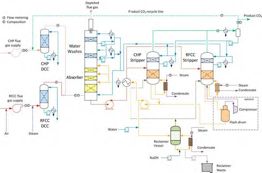
Figure 1: Schematic illustration of the TCM DA amine plant.
2.1 MEA campaign overview
The MEA test campaign was conducted from 06/07/2015 to 17/10 2015. During the total 1960 hours of operation a wide range of operational process conditions were executed and a total of 4941 tons of CO2 was captured. The variation of gas and solvent flow rates and stripper bottom temperatures are presented in Figure 2, while further details on typical operating process conditions are presented in Table 1 of Gjernes et al. (2017) [7]. The test campaign was operating on 30 ± 2 wt% MEA and the ranges of the lean and rich CO2 loadings during the campaign was 0.19 – 0.29 and 0.46 – 0.53 mol CO2/mol MEA, respectively. The majority of the campaign was operated with CHP flue gas; however, for a shorter period of 9 days from 16/09/2015 to 24/09/2015 it was operated on a mixture of CHP and RFCC gas, as indicated in Figure 2. Thermal reclaiming was performed towards the end of the campaign, after 1838 hours of operation. Reclaiming was performed for 92 hours, and the plant was run for an additional 28 hours after the reclaiming period before the campaign was concluded 17/10/2015.
Figure 2: Overview of the daily gas and solvent flow rates and stripper temperatures during the MEA test campaign.
3. Solvent degradation during the test campaign
3.1 Process conditions that influenced solvent degradation
The MEA test campaign was conducted by executing a wide range of process conditions with frequent operational set-point changes. Such a shifting operating environment might accelerate solvent degradation. The average stripper bottom temperature was 120 °C, with a maximum of 122.5 °C. Superheated MP steam in the temperature range of 130 – 150 °C was used as heat source in the stripper reboiler. The reboiler skin temperature for which the solvent is exposed to, can therefore be assumed to be around 130°C. The solvent will undergo thermal degradation when exposed to temperatures at this level.
The majority of the campaign was operated with CHP flue gas. However, as part of specific mist testing where the aim was to induce formation of aerosols and study its effect on emissions, the plant was operated on a mixture of CHP and RFCC gas [8]. The mist testing where more specifically conducted by;
- Increasing the concentration of CO2 in the feed flue gas up to 12 vol% by recycling parts of the captured CO2 to the absorber flue gas inlet.
- Mixing portions of the RFCC flue gas with the CHP flue gas.
Up to 10 % mixing of RFCC gas in CHP gas was tested. Typical CHP and RFCC gas concentrations downstream the DCCs are presented in Table 1. As seen in the table, the CHP flue gas contains significant amounts of oxygen which causes oxidative degradation. Exposure to higher concentrations of CO2 and RFCC gas impurities during the mist testing accelerated the rate of solvent degradation. Further, metal particulate material present in the RFCC gas might have contributed as catalysts for oxidative degradation.
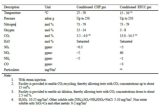
Table 1: Typical CHP and RFCC flue gas conditions downstream DCC conditioning at TCM DA.
3.2 The impact of process design on solvent degradation
As mentioned above, the main factors causing solvent degradation was elevated operating temperature in the stripper section and exposure to oxygen and contaminants in the flue gas. The effect of thermal and oxidative degradation will not only depend on these factors themselves, but also on the solvent residence times in the sections of the plant where these factors are significant, i.e. the part of the plant where the solvent is exposed to higher temperatures and oxygen and gas contaminants.
The hot solvent inventory (desorber packing, desorber sump, reboiler, hot part of the lean/rich cross heat exchanger and the hot lean and rich solvent piping) calculated for CHP baseline operating conditions are presented in Table 2. For details about the CHP baseline operating conditions it is referred to Faramarzi et al. (2017) [9]. The total of 13.4 m3 hot solvent inventory is quite significant and corresponds to about 35% of the total solvent inventory. The corresponding solvent residence time is about 20 minutes for CHP baseline operating conditions. The main contributor to the hot solvent inventory is clearly the rather long hot lean solvent pipe, which contributes to 60% of the total hot solvent inventory. The reboiler itself has a rather low solvent residence time; however, the beforementioned reboiler skin temperature of about 130 °C might also contribute to significant thermal degradation as degradation increases exponentially with the temperature.
The solvent inventory exposed to oxygen and the corresponding oxygen exposure time is also presented in Table 2. It is expected that the largest effect of oxygen exposure is seen in the absorber packing, where the actual inventory and exposure time is estimated to about 8 m3 and 12 minutes, respectively, considering CHP baseline operating conditions. This abovementioned exposure time is also relevant for flue gas contaminants when operating on CHP/RFCC gas mixture.
In order to minimize solvent degradation it is clearly of interest to perform plant design such that the exposure times to oxygen and elevated temperatures are limited. For scale-up purposes it is therefore of specific importance to minimize solvent hold-up in hot parts of the plant.
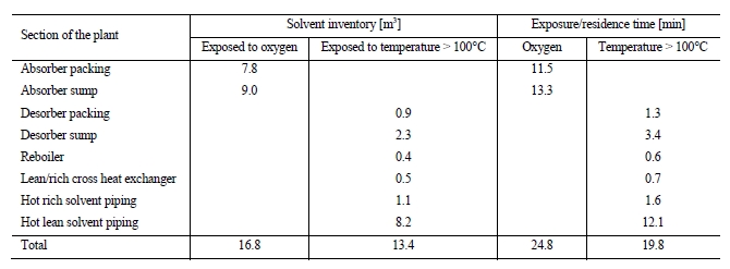
Table 2: Estimated solvent inventory and residence times for solvent exposed to oxygen and elevated temperatures based on CHP baseline operating conditions (for details about the CHP baseline conditions it is referred to Faramarzi et al (2017) [9].
3.3 Monitoring of solvent degradation
Solvent degradation was observed and monitored by a number of parameters during the test campaign. Lean and
rich solvent samples were frequently withdrawn for solvent analysis. The analytical methods are described by
Morken et al (2017) [10]. Firstly the physical properties of the solvent changed during the campaign as shown by the increase of solvent viscosity in Figure 3. The viscosity was measured in TCM DA lab and reported at two different temperatures (30°C and 60°C) and a clear increase of about 50% is observed from the test campaign start until reclaiming started on 12/10/2015.
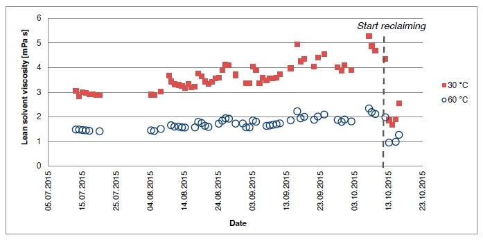
Figure 3: Change in solvent viscosity during the MEA test campaign.
A clear observation of solvent degradation was also the change of solvent color during the test campaign. The fresh 30 wt% MEA solvent started out as a clear liquid, which changed color quite fast after contact with flue gas. The solvent became gradually darker during the campaign, until it reached the dark brown color illustrated by the third sample glass from 11/10/2015 in Figure 4.
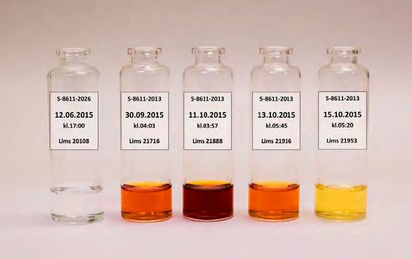
Figure 4: Picture of solvent samples taken during the campaign. The color change indicates solvent degradation.
Further, the level of volatile degradation products in the gas phase increased significantly during the period of Mist testing. Morken et al (2017) presents detailed results regarding ammonia emissions, which is associated with presence of ammonia in the solvent originating from solvent degradation [10]. Emission of ammonia is also highly dependent on operating conditions; however the observed build-up of ammonia in the solvent is regarded as a clear sign of solvent degradation.
Heat stable salts started building up in the solvent as shown in Table 3 before it reached a maximum of 0.203 mol/kg just before reclaiming started on 12/10/15. More detailed results concerning HSS analysis are presented by Morken et al (2017) [10]. The concentration of main degradation products was also monitored continuously and shows a significant increase as the test campaign progressed. It is referred to Morken et al (2017) for details [10].
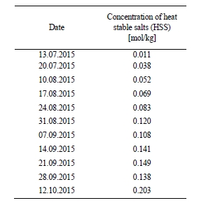
Table 3: Total concentration of heat stable salts (HSS) during the campaign.
Additional parameters which are important to monitor during operation of the amine plant are solvent foaming tendency and metal ion concentration. The latter gives indications of plant corrosion and was also monitored during the test campaign. The results are presented by Hjelmaas et al. (2017) [11].
4. Reclaiming procedure and operational experience
The reclaimer was operated in a semi-continuous operation mode, meaning that solvent was continuously fed to the reclaimer vessel, while the reclaimer waste was allowed to accumulate and was only disposed at the end of the test campaign. The process was operated continuously for 3 days with exception of one unexpected plant stoppage for about 3 hours on the 13/10/2015.
The reclaimer vessel was initially filled with water. Water circulation and steam heating was started before the solvent feed to the reclaimer vessel. The rather large volume of initial water evaporated during the reclaiming operation and resulted in dilution of the solvent as shown in Figure 5.
The reclaimer liquid was circulated in the reclaiming system loop through the steam heat exchanger at a circulation rate of approximately 165 m3/h. No boiling occurs in the steam heater, but the liquid flashes when it enters the evaporator vessel. The evaporating level was controlled by adjusting the steam rate supply. As the liquid became more concentrated, its boiling temperature increased and the rate of evaporation was reduced. The percentage of degradation products in the reclaimer, and the resulting temperature were slowly increasing. Upon reaching high temperature, high viscosities and high amounts of precipitates, the reclaimer feed was stopped.
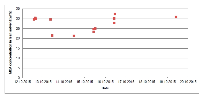
Figure 5: MEA concentration in the lean solvent during reclaiming.
4.1 Solvent and water feed rate
The reclamation unit was fed with a continuous slip stream of the lean amine solvent from downstream the stripper. The reclaimer was also fed simultaneously with water in order to control the boiling temperature of the reclaimer fluid below 160 °C. Figure 6 presents the solvent and water flow rates along with the reclaimer liquid temperature.
The solvent slip stream corresponded to 4 – 5 % of the lean solvent circulation and was up to a maximum of about 3 000 kg/h as illustrated in Figure 6. A total accumulated amount of 46 000 kg solvent was fed to the reclaimer during the whole period of 3 days. This corresponds to about 110 % of the total solvent inventory.
4.2 Steam consumption
The reclaimer heat duty variations were according to the changing amount of the lean solvent slip stream directed to the reclaimer vessel. As shown in Figure 7, in order to vaporize MEA in the reclaimer a significant amount of heat was required. At times, the amount of heat used for reclaiming was almost equal to the heat used to regenerate the solvent in the stripper. As reclamation of MEA is energy intensive, it is important to optimize the amount of lean amine slip stream sent to the reclamation unit. However, as shown in Figure 6 the flow of slip stream varied due to the fluctuations in the process conditions and it was not possible to achieve a constant flow during the reclaiming procedure.
The reboiler heat duty increased significantly when the reclaimer was brought on stream and then plateaued at about 2 500 kW. This was due to the large amount of water that was initially added to reclaimer unit, which evaporated from the reclaiming vessel and caused dilution of the solvent. The concentration of MEA was consequently reduced to about 21 wt% as shown in Figure 5. Thus the amount of water to be boiled off in the stripper was much larger, causing higher energy numbers.
The reclaimer liquid circulation and steam heating continued for 2 days after the solvent feed was stopped in order to evaporate as much as possible of the useful MEA solvent and concentrate the waste.
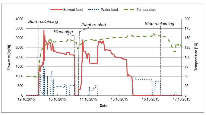
Figure 6: Reclaimer solvent slip stream, water feed rate and reclaimer liquid temperature.
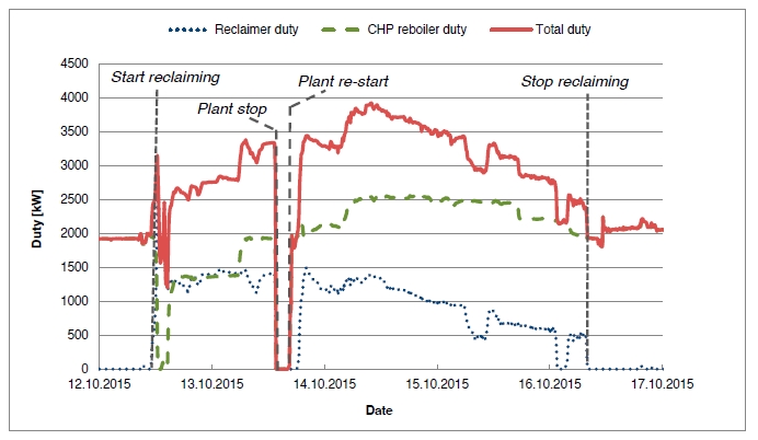
Figure 7: Steam consumption during reclaiming.
4.3 Dosage of NaOH
Aqueous solution of 50 wt% NaOH was added to the reclaimer vessel via the reclaimer liquid circulation loop in order to stabilize anions of amine heat stable salts by converting them to sodium salts and liberating the amine according to Reaction (1). The recovered amine and water vapor was returned to the stripper sump.
A dosage rate of 3 L NaOH/m3 solvent was applied during reclaiming based on previous experience at TCM DA. In total 227 liters 50% NaOH was added, which corresponds to 4299 mol Na+.
According to Reaction (1), the stoichiometric ratio of NaOH to HSS should ideally be 1:1. This is a very rough estimate since the actual ratio depends on the electrical charge of the anions. The concentration of HSS components was 0.203 mol MEA-eq/kg solvent at the point of reclaiming start 12.10.15 (see Table 3). With a total solvent inventory of 40 800 kg in the plant at the time, this corresponds to 8282 mol HSS. A stoichiometric check shows excess HSS compared to NaOH, which might cause additional MEA loss in the reclaimer waste.
4.4 Reclaimer waste
After the reclaiming operation was concluded the majority of the concentrated waste was drawn off to the flushing line and passed through the sea water cooler to the IBC (Intermediate Bulk Container) drainage system. The reclaimer fluid was quite concentrated and viscous at the time, thus some water was added in order to dilute the waste and enable unloading of the vessel. The total concentrated waste was collected in IBCs and added up to a total of about 6 m3. This corresponds to about 1.3 kg reclaimer waste/ton CO2 captured during the overall campaign, which is well below reported numbers in the literature. Further, the reclaiming process was initiated when HSS concentration reached 0.203 mol/kg, as beforementioned. The actual necessity of reclaiming at this level of HSS must be considered based on the actual solvent condition and potential plant corrosion issues, i.e. at this moment the reclaiming campaign was not necessary but rather conducted for demonstration purposes in the test campaign. The waste/ton CO2 capture would thus be even lower in an actual necessary reclaimer case. The reclaimer vessel and piping was afterwards flushed with water.
5. Efficiency of thermal reclaiming
In order to investigate the reclaiming efficiency and demonstrate how the solvent quality is recovered and maintained by the reclaiming process, samples were frequently taken from the lean amine solvent, the reclaimer liquid and reclaimer vapor. The samples were analyzed for MEA, degradation products, HSS and metals, and the results are summarized in Table 4.
The concentration of degradation products in lean amine was analyzed throughout the test campaign and the results are presented by Morken et al (2017) [10]. Figure 8 below shows the concentration of degradation products in the lean amine solvent during the reclaiming operation. It is seen that the degradation products is efficiently cleaned from the lean amine and about 95% percent of the degradation products was removed. A small increase in concentration from day three indicates that degradation is significant during reclaiming, likely due to thermal degradation due to operation at elevated temperatures inside the reclaimer vessel.
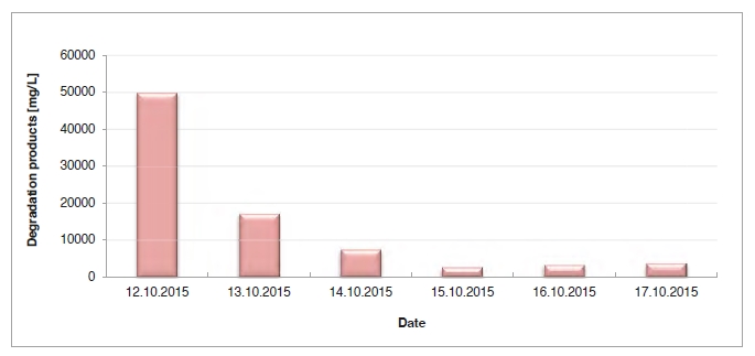
Figure 8: Concentration of degradation products (D-mix) in lean amine during reclaiming.
A very similar trend is seen for the concentration of metal elements iron (Fe), Nickel (Ni) and Chromium (Cr) in
Figure 9 below. The concentration is reduced by more than 95% after reclaiming.
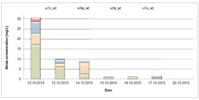
The trends for heat stable salts in the lean solvent, reclaimer liquid and the reclaimer vapor are shown in Figure 10. Again, the concentration of HSS in lean amine is rapidly reduced to less than 5% of the start concentration, as shown by the blue columns in the graph. The accumulation of HSS in the reclaimer liquid is also clearly seen by the red columns. HSS could not be detected in the reclaimer vapor return to stripper, as expected. Figure 11 presents the concentration of MEA, NaOH and HSS in the reclaimer liquid during the reclaiming process. Most of the MEA is evaporated during the period as seen in the figure. HSS and Na+ is accumulated, however MEA seems to be in excess, also at the end of the reclaiming.
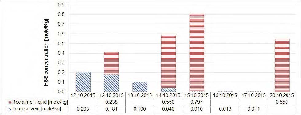
Figure 10: Concentration of HSS in lean amine and the reclaimer liquid.
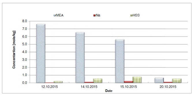
Figure 11: Concentration of MEA, NaOH and HSS in the reclaimer liquid.
The color of the solvent changed back to a lighter color after reclaiming as illustrated by the fifth sample glass from 15/10/2015 in Figure 4. Based on analysis of the reclaimer waste and assessment of the total MEA inventory in the plant before and after reclaiming, it is estimated that about 500-550 kg MEA was lost to waste during reclaiming. This corresponds to 4% of the total inventory (according to Table 4) and 0.11 kg MEA/ton CO2 captured.
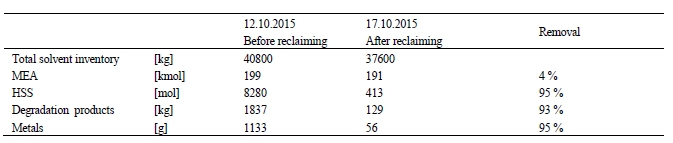
Table 4: Amount of HSS, degradation products and metals removed from the solvent and MEA lost in reclaimer waste.
6. Solvent performance after reclaiming
After the reclaiming operation had been concluded the plant was operated for another 28 hours at a flue gas flow rate of 47,000 Sm3/h. Two test cases were conducted during this period, and these are used for comparison to other similar tests conducted previously in the campaign with a fresh solvent. The two test cases after reclaiming is designated “T4” and “T5”, while the optimum energy case with the use of anti-foam (case 2B6) from previously in the campaign is used for comparison. The total operating hours at the point in time when case 2B6 was conducted was approximately 950 hours. The overall 2015 MEA campaign and the entire specific test series carried out to investigate the capture plant performance is described by Gjernes et al. (2017) [7].
Figure 12 summarizes the operation before and after reclaiming. T4 and T5 were operated with 24 and 18 m absorber packing height, respectively. During T4 the amine plant was a bit unstable while there were stable conditions during T5. Case 2B6 was operated with 24 meters of packing height. The plant performance after reclaiming was comparable to the optimum performance achieved earlier in the campaign and there were no significant indications of reduced solvent quality.
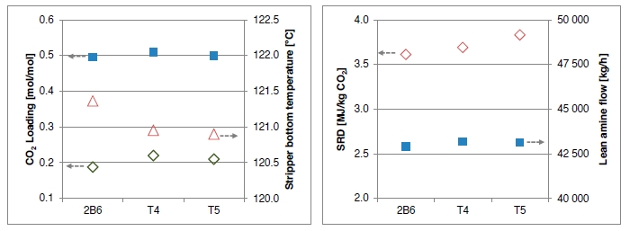
Figure 12: Results for test cases 2B6, T4 and T5: To the left rich- (squares) and lean-loading (diamonds) and stripper bottom temperature (triangles) and to the right SRD (diamonds) and lean amine flow (squares).
7. Discussion and future work
Monitoring the amine concentration and CO2 loading is very important for optimal operation. At TCM DA the solvent concentrations are mainly followed on a daily basis with manual samples and analysis. Further, a number of analyzers are available for real-time online monitoring, i.e. conductivity, density and pH analyzers. These online results can be correlated to enable a closer follow-up of the solvent condition.
As an effect of reclaiming start-up, the solvent in the main process was diluted by water evaporating from the reclaimer vessel. In future campaigns, extra care will be taken not to disrupt the main process during reclaiming. The deviation in solvent concentration could have been corrected at an earlier stage with an online estimate of solvent concentration.
The reclaiming environment is very harsh to the solvent due to high temperatures (up to 160 °C). The elevated temperatures represent a risk of additional thermal degradation. Care must therefore be taken in order to limit the residence time of the reclaimer solvent and thereby unnecessary degradation. Thus frequent manual solvent sampling or online analyses are required in order to monitor the progress of reclaiming and terminate the reclaiming process when the target is reached. In this test campaign it was very successfully demonstrated a 95 % cleaning efficiency when circulation a 4-5 % slip stream through the reclaimer for three days, which added up to an accumulated reclaimed volume of about 110% of the total solvent inventory.
The total HSS analysis indicates that the amount of NaOH added during reclaiming was on the stoichiometric low side to limit the MEA loss in the reclaimer waste. It is therefore reason to believe that additional MEA was lost in HSS to the waste. Thus, the total MEA loss of 4% could be reduced even further by optimizing the NaOH dosage. However, the actual effect of NaOH addition on MEA release from HSS should be investigated more in detail.
There is little information available in the literature that addresses how the build-up of impurities impacts the energy demand for regenerating MEA in the stripper i.e. reboiler heat duty. However, the density and viscosity of the solvent increased with the increasing level of contaminants as discussed in Section 3. This will cause reduction of the solvent heat transfer coefficient and consequently the heat transfer efficiency in the reboiler. The impact of accumulation of the contaminants on the specific heat capacity of amines is also very little addressed in the literature. However, it is expected that degraded MEA has higher specific heat capacity than MEA which in turn could increase the sensible heat needed to regenerate the solvent in the stripper. It is recommended to investigate these effects in the future.
As the amine plant was only operated for 28 hours after solvent reclaiming, a very limited investigation of the effect of removing the aqueous phase contaminants on the energy requirement of the stripper reboiler was performed. In future tests, sufficient time should be allowed to investigate in detail and compare the solvent performance at the beginning of the test campaign to the performance just before reclaiming and just after reclaiming.
In order to further optimize the process and reduce disposal problems both the reclaiming procedure itself and the collection and drainage of the reclaimer waste can be improved. The rapid cleaning of the lean solvent suggests running the reclaimer more frequently for shorter time periods (for example 12 hours a week) as one option to avoid degraded solvent to accumulate in lean amine. In this way the acceleration of degradation reactions could also be minimized. The draining and flushing operation can be improved by using less water or even small amounts of steam for keeping the reclaimer vessel fit for purpose. This will reduce the amounts of waste.
8. Conclusions
A test campaign with 30 wt% MEA has been conducted for a total of 1960 hours at the CO2 Technology Centre Mongstad. The present paper discusses main causes of solvent degradation and various parameters for monitoring degradation products. Further, the effect of process design and operating conditions on solvent degradation is discussed, and thermal reclaiming is evaluated as a technique for removal of degradation products and other contaminants in the MEA solution.
The solvent condition was closely monitored during the test campaign and several observations such as increasing solvent viscosity and darker solvent color indicated solvent degradation. Solvent exposure to oxygen and flue gas contaminants in the absorber and operation at elevated temperatures (above 100 °C) in the stripper section are highlighted as main causes for degradation. When performing scale-up to commercial CO2 capture units it is recommended to minimize the hot solvent residence time in the plant, in order to minimize solvent degradation.
Thermal reclaiming has demonstrated an efficient clean-up of the MEA solvent. The cleaning efficiency was about 95% with respect to degradation products, HSS and metal elements. The solvent viscosity returned to normal values and the solvent color was normalized to a clearer and more yellow appearance. The quality recovery of the solvent was further assessed by an evaluation of the capture process after the reclaiming was concluded by comparing the solvent performance to results obtained at earlier stages of the test campaign and there were no significant indications of reduced solvent quality.
Acknowledgements
The authors gratefully acknowledge the staff of TCM DA, Gassnova, Statoil, Shell and Sasol for their contribution and work at the TCM DA facility. The authors also gratefully acknowledge Gassnova, Statoil, Shell, and Sasol as the owners of TCM DA for their financial support and contributions.
References
- Dumée L, Scholes C, Stevens G, Kentish S. Purification of aqueous amine solvents used in post combustion CO2 capture: A review. International journal of Greenhouse Gas Control 10 (2012): 443-455.
- Abdi MA, Golkar MM. Improve contaminant control in amine systems. Hydrocarbon Processing 63 (2011): 102C – 102-I.
- IEAGHG, “Evaluation of Reclaimer Sludge Disposal from Post-Combustion CO2 Capture”, 2014/02 (March 2014).
- Wang T, Hovland J, Jens, KJ. Amine reclaiming technologies in post-combustion carbon dioxide capture. Journal of Environmental Science 27 (2015): 276 – 289.
- Kohl AL, Nielsen RB. Gas purification. Gulf publishing Company, Houston, Texas, USA, 5th edition (1997).
- Nurrokhmah L, Mezher T, Abu-Zahra MRM. The evaluation of monoethanolamine-based CO2 post-combustion capture process waste handling approaches considering the regulations in UAE. Energy Procedia 37 (2013): 751 – 758.
- Gjernes E, Pedersen S, Cents T, Watson G, Fostås BF, Shah MI, Lombardo G, Desvignes C, Flø NE, Morken AK, de Cazenove T, Faramarzi L, Hamborg ES. Results from 30 wt% MEA performance testing at the CO2 Technology Centre Mongstad. Energy Procedia (GHGT-13), Forthcoming 2017.
- Lombardo G, Fostås BF, Shah MI, Morken AK, Hvidsten OA, Mertens J, Hamborg ES. Results from aerosol measurement in amine plant treating gas turbine and residue fluidized catalytic cracker flue gases at the CO2 Technology Centre Mongstad. Energy Procedia (GHGT- 13), Forthcoming 2017.
- Faramarzi L, Thimsen D, Hume S, Maxson A, Watson G, Pedersen S, Gjernes E, Fostås BF, Lombardo G, Cents T, Morken AK, Shah MI, de Cazenove T, Hamborg ES. Results from MEA testing at the CO2 Technology Centre Mongstad: Verification of baseline results in 2015. Energy Procedia (GHGT-13), Forthcoming 2017.
- Morken AK, Pedersen S, Kleppe ER, Wisthaler A, Vernstad K, Ullestad Ø, Flø NE, Faramarzi L, Hamborg ES. Degradation and Emission Results of Amine Plant Operations from MEA Testing at the CO2 Technology Centre Mongstad. Energy Procedia (GHGT-13), Forthcoming 2017.
- Hjelmaas S, Storheim E, Flø NE, Thorjussen ES, Morken AK, Faramarzi L, de Cazenove T, Hamborg ES. Results from MEA amine plant corrosion processes at the CO2 Technology Centre Mongstad. Energy Procedia (GHGT-13), Forthcoming 2017.