
1. Optimum Conditions and Maximum Capacity of Amine-Based CO2 Capture Plant at Technology Centre Mongstad (2024)
Shahin Haji Kermani 1, Koteswara Rao Putta 2 and Lars Erik Øi 1,*
1Department of Process, Energy and Environmental Technology, University of South-Eastern Norway, Kjølnes Ring 56, 3918 Porsgrunn, Norway
2Technology Centre Mongstad, 5934 Mongstad, Norway
*Author to whom correspondence should be addressed.
ChemEngineering 2024, 8(6), 114; https://doi.org/10.3390/chemengineering8060114
Abstract
Using amine-based solutions is a mature method for CO2 capture. This study simulates this process at Technology Centre Mongstad (TCM) using a rate-based model in Aspen Plus. The main purpose is to develop a rigorous model for TCM and find the operation limits, maximum utilization capacity, and maximum achievable CO2 removal efficiency at the plant. The model accuracy is verified by using different scenarios from the test campaign reports at TCM with three main configurations: Combined Heat and Power flue gas, Refinery Residue Fluid Catalytic Cracker flue gas, and cold rich-solvent bypass. The deviation between the experimental data and simulation results is compared. The model shows better accuracy with more detailed input data and accurate practical parameters. The verified model is used with all the TCM configurations to simulate the plant. Aspen Exchanger Design and Rating is also used to design real heat exchangers. To avoid flooding, the maximum gas flow to the absorber column is 52,000 Sm3/h. There is a maximum reboiler duty of 8.4 and 3.4 MW for the Residue Fluid Catalytic Cracker and the Combined Heat and Power flue gas strippers, respectively. The optimum operating condition to achieve a CO2 removal efficiency of 90% after amine lean loading adjustment, using maximum gas flow, both strippers, and 15% rich-solvent bypass, gives a total specific reboiler duty of 3.0 MJ/kgCO2. By using a maximum amine flow rate of 230 ton/h, a CO2 removal efficiency of 98% can be achieved. The optimum modification gives a bypass fraction of 19% and a specific reboiler duty of 3.63 MJ/kgCO2.
Keywords: TCM; Aspen Plus; CO2 capture; MEA; simulation; limitation
1. Introduction
Technology Centre Mongstad (TCM) is the world’s largest and most flexible test center for developing and improving CO2 capture technologies and a leading competence center for carbon capture. It is located at one of Norway’s industrial facilities, and it was initiated in 2006 when the Norwegian government and Statoil (now Equinor) agreed to establish the world’s largest full-scale CO2 capture and storage project [1]. Lots of performance data on different scenarios at the TCM test facility using monoethanolamine (MEA) are available. It is necessary to have good and robust simulation models to analyze the process behavior.
Several projects have been performed at the University of South-Eastern Norway (USN) on process simulations of amine-based CO2 capture. Most of the simulations have been performed with the programs Aspen HYSYS and Aspen Plus.
The focus of this project is to perform a literature review on the performance data of amine-based CO2 capture using MEA at TCM, develop a rate-based model in Aspen Plus on the CO2 capture process for the TCM plant operational data, verify the model with previous test campaigns, extend and modify the model with the advanced configurations at the TCM plant to find the maximum utilization capacity of the installed equipment and the operation limits, and optimize the operating condition to achieve the maximum CO2 removal efficiency by using the maximum gas and amine flow rate and advanced configurations at TCM.
Outline of this paper:
In Section 2, there is a thorough literature review and a problem description.
In Section 3, the simulation model and methodology are presented, including the different simulation tools and necessary calculations. Simulation and model specification, including property methods, together with the equipment specification of the simulated equipment, are presented in this section.
Section 4 presents the model validation with different scenarios and performance data from the previous test campaigns and compares them with the simulation results.
In Section 5, the verified rate-based model is extended to simulate the TCM plant with a more detailed heat exchanger simulation and using a specific scenario named MHP. Moreover, simulation modification and the TCM plant utilization limitations for each piece of the installed equipment are discussed and obtained in this chapter. Optimization of the model to obtain maximum plant capacity and the operating condition to achieve the maximum CO2 removal efficiency are also presented in this chapter.
Section 6 presents a summary of the practical TCM plant limits and modifications, as well as a discussion about the model accuracy, plant optimization, and energy consumption. Recommended future works are also mentioned in the last section of the section.
Section 7 presents the conclusion of this work.
2. Background
2.1. CO2 Emission and Climate Change
Carbon dioxide (CO2) is one of the major greenhouse gases, and it has been emitted in massive quantities in the last decades. As a result, over thirty billion tons of CO2 is added to the atmosphere each year, which can bring many environmental issues [2].
2.2. Amine Solution Technology
An amine-based solution is currently the most mature and cost-effective way to remove CO2 from industrial flue gases. Other alternative CO2 removal processes have been evaluated by Li et al. [2]. In that overview, several patented processes including solid-sorbent-based, solvent-based, and membrane-based processes were reviewed. In the amine-based method, CO2 from the flue gas is absorbed and captured into an aqueous amine solution. The rich amine, including absorbed CO2, leaves the absorber at the bottom and is then piped to the desorber column or stripper to be heated with steam. As a result, CO2 is released from the amine solution, and the regenerated amine is recirculated to the absorber. Figure 1 shows the schematic of an amine scrubbing unit [3].
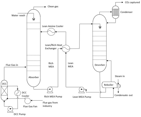
Figure 1. Schematic of amine scrubbing unit [3].
The most conventional amine for the CO2 capture process is monoethanolamine (MEA), with the formula H2NC2H4OH, and it is considered in this study.
It should be noted that there are also different alternatives for process optimization, for example, lean vapor compression (LVC), which can result in energy reductions in some cases. The lean amine from the stripper’s bottom is flashed at a lower pressure than the stripper pressure, and it is compressed and recycled to the stripper. The CO2 loading (mole CO2/mole MEA) in lean amine will decrease, thus reducing the required amine flow rate or increasing the CO2 removal efficiency in the absorber [4]. Another example is absorber intercooling, in which a portion of the semi-rich-solvent is cooled in the middle of the absorber by removing, external cooling, and injecting to reduce the temperature and increase solvent absorption capacity. This enhances the driving force of CO2 transfer at the bottom of the column, which increases the solvent’s absorption capacity, resulting in a lower solvent circulation rate [5].
2.3. Process Description at TCM
Technology Centre Mongstad (TCM) is a highly flexible plant aimed to accommodate a variety of technologies with the capabilities of treating flue gas streams. The plant generally works with two different types of flue gas: Combined Heat and Power (CHP) and Refinery Residue Fluid Catalytic Cracker (RFCC). In general, CHP flue gas has a lower concentration of CO2 in comparison with RFCC flue gas. Figure 2 shows the process flow diagram for CO2 capture at the TCM plant [6].
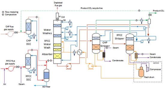
Figure 2. A process flow diagram of the TCM Amine plant with the illustration of the two different flue gases (CHP and RFCC), as well as the available strippers [6]. The dotted line is the limit for the vapor recompression part which is not included in the simulations in this work.
2.4. Literature Review of Simulation of CO2 Capture Based on Performance Data
Comparisons and fitting of simulation models with performance data for amine-based CO2 capture are relatively new. The first references mentioned here are from 2009. Luo et al. [7] used sixteen data sets from four different pilot plant studies and validated the data with simulations in four different simulation tools (Aspen Plus equilibrium-based, Aspen Plus rate-based, ProMax, ProTreatTM, and CO2SIM). They concluded that the reboiler duties, concentrations, and temperature profiles were less predictable, and all the simulation tools were able to present reasonable predictions on the overall performance of the CO2 absorption rate. Zhang et al. [8] developed, in 2009, a rate-based model in Aspen Plus based on fitting parameters to performance data from a test rig at the University of Texas. In the Aspen Plus rate-based model, there are several available correlations to estimate the mass transfer numbers on the gas side and the liquid side, the heat transfer number, the interfacial area, and the holdup. Tobiesen et al. [9] developed a rate-based model of acid gas absorption and a simplified absorber model. They validated the models against mass transfer data obtained from a 3-month campaign in a laboratory pilot-plant absorber. It was found that the simplified model was satisfactory for lower CO2 loading, while the rigorous model had a better fit for higher CO2 loading. Ying Zhang and Chau Chen [10] at the University of Kaiserslautern simulated 19 data sets of CO2 absorption in MEA with rate-based and equilibrium-based models. Their result shows that the rate-based model yields reasonable predictions, while the equilibrium-based model fails to predict these key performance variables. Øi [11] compared Aspen HYSYS (version 12, Aspen Technology, Cambridge, MA, USA) and Aspen Plus (rate-based and equilibrium) (version 12, Aspen Technology, Cambridge, MA, USA) simulations of CO2 capture with MEA. The conclusion was that there were small deviations in the equilibrium-based model in Aspen HYSYS and Aspen Plus. Øi found larger deviations between the equilibrium-based calculations and the rate-based calculations.
Several papers have been published where flowsheet modifications of the straightforward absorption and stripping process are presented and simulated. Cousins et al. (2011) analyzed process flowsheet modifications for energy-efficient CO2 capture. They suggested modifications, including split flow, rich bypass, vapor recompression, and intercooling, using rate-based simulation. Finding an optimum ratio of the rich-solvent bypass was also conducted by Cousins [12]. Kvam [13] compared Aspen Plus (rate-based and equilibrium-based) and Aspen HYSYS (Kent–Eisenberg and Li–Mather) simulations for CO2 capture with MEA. His main goal was to compare the energy consumption of a standard process with vapor recompression and with vapor recompression with a split stream. Aromada et al. [14] studied how a reduction in energy consumption can be achieved by using alternative configurations. They simulated a standard vapor recompression and vapor recompression combined with a split stream in Aspen HYSYS for 85% amine-based CO2 removal. The results show that it is possible to reduce energy consumption with both vapor recompression and vapor recompression combined with split-stream processes. Rehan et al. [15] studied the performance and energy savings of installing an intercooler in a CO2 capture system. They used Aspen HYSYS to simulate the CO2 capture model. The results show slightly improved CO2 recovery performance and the potential for significant savings in MEA solvent loading and energy requirements by installing an intercooler in the system. Arshad and Alhajaj [5] studied techno-economic evaluations of advanced MEA-based CO2 capture process configurations. They validated and used a rigorous rate-based model in Aspen Plus, including intercooling, rich-solvent bypass, and lean vapor recompression, with a focus on energy and cost reductions. A combination of these three gave the lowest levelized cost of CO2 capture.
Test Center Mongstad (TCM) is the world’s largest test facility for amine-based CO2 capture. The first performance data available from the plant were from 2013 and published later by Thimsen et al. [16]. Hamborg et al. [17] published a paper with the results from the MEA testing at TCM during the 2013 test campaign. The paper shows the CO2 removal efficiency, temperature measurements, and experimental data for the process. Erik Gjernes et al. [18] published the results from 30 wt% MEA performance testing at TCM. The main objective was to demonstrate and document the performance of the plant. Leila Faramarzi et al. [19] published a paper with the results from the MEA testing at TCM during the 2015 test campaign. The paper shows CO2 removal efficiency, temperature measurements, and experimental data for the process. Shah et al. [20] presented the results of the advanced amine plant process configuration at TCM for six different cases of RFCC flue gas with 30 wt% MEA. The advanced configuration, in addition to the conventional configuration, consists of a three-stage water wash system, an online sampling system tolerating aerosol, and operational parameters. The result shows reduced SRD and reduced aerosol-based amine emissions. Shah also suggested having a rich bypass of the solvent for further reduction in SRD. Meuleman et al. [21] discussed the results of CO2 capture at TCM by using ION Engineering’s advanced solvent on eight different RFCC and five different cases of CHP flue gases from the adjacent Statoil refinery, with different CO2 concentrations from 3.6% to 15%. Fosbøl et al. [22] presented the process variables data from the lean vapor compressor campaign at TCM. They tested 16 cases with various parameters, such as LVC pressure, solvent flow, inlet flue gas CO2 concentration, and stripper pressure, to create knowledge on the process performance of LCV on the CO2 capture efficiency and energy profile of the TCM plant. Hume et al. [23] presented the results from MEA testing at TCM with RFCC flue gas with a high concentration of CO2 (13–14%). These data can provide a new baseline case for 30 wt% MEA solvent in higher concentration flue gas capture cases.
Several papers have been published based on comparisons of simulations with performance data at TCM. Larsen [24] simulated a rate-based Aspen Plus model and compared the results with experimental data from TCM. Larsen found that the TCM model used in Aspen Plus was in general agreement with the experimental data. She also found that temperature and loading profiles are similar to the experimental data by adjusting parameters. Desvignes [25] simulated conditions for high concentrations of MEA and compared them with performance data at TCM. Zhu [26] simulated an equilibrium model in Aspen HYSYS based on the data from the TCM 2013 campaign published by Hamborg et al. [17]. He adjusted the Murphree efficiency to fit the CO2 removal efficiency and temperature profile from the experimental results. Zhu found that a linear decrease in Murphree efficiency from top to bottom can give a good temperature prediction. Sætre [27] simulated seven sets of experimental data from the amine-based CO2 capture process at TCM with Aspen HYSYS (Kent–Eisenberg and Li–Mather) and Aspen Plus (rate-based and equilibrium). He found that it is possible to fit a rate-based model by adjusting the interfacial area factor and an equilibrium-based model by adjusting the Murphree efficiency factor. Both Aspen HYSYS and Aspen Plus can give good results if there are only small changes in the parameters. Øi et al. [28] compared four sets of experimental data from the amine-based CO2 capture process at TCM, with different equilibrium-based models in Aspen HYSYS and Aspen Plus, as well as a rate-based model in Aspen Plus. They concluded that equilibrium and rate-based models perform equally well in fitting the performance data and in predicting the performance at different conditions. Fagerheim [29] used the stage efficiency profile developed by Zhu [26] to simulate and develop other profiles in Aspen HYSYS. She concluded that the profiles can be fitted to different tests by using a Murphree efficiency factor. Five of the cases documented by Sætre [27] were used in her study. She also compared the result with rate-based model simulations using Aspen Plus. Sæter [30] simulated the results of pilot plant data from TCM for both high and low CO2 exhaust gas inlet concentrations in both a rate-based model in Aspen Plus and an equilibrium-based model in Aspen HYSYS. In his work, the rate-based model was fitted by only changing the liquid hold-up factor, and in the equilibrium-based model, the Murphree efficiency was specified for 24 and 18 stages in the absorber column to fit the performance data and the temperature profile. A Murphree efficiency factor was used to fit other performance data in different scenarios. Montanes et al. (2018) and Bui et al. (2020) [31,32] have fitted dynamic models in Aspen HYSYS and Aspen Plus to time-dependent performance data. Shah et al. [6] conducted a cost-reduction study for MEA-based CO2 capture at TCM. During this campaign, the main focus was on thermal energy optimization at different flue gas flow rates through the absorber column and MEA emissions, with a target for reduced CAPEX and OPEX. New options, such as rich-solvent bypass to stripper overhead, were also conducted in their tests. Putta et al. [33] have validated a rate-based Aspen Plus model by fitting it to steady-state performance data in a scenario from TCM. They performed a CO2 Capture Process Cost estimation baseline by considering all essential elements of the CO2 capture process at TCM.
2.5. Problem Description
In this paper, a rate-based model in Aspen Plus is used to simulate the TCM plant, including rich-solvent bypass. The heat exchangers, the reboilers, and the condenser are designed using Aspen Exchanger Design and Rating (Aspen EDR) v.12 as the real equipment in the plant. The accuracy of the model is tested by experimental data from previous test campaigns at TCM. Moreover, the plant limitations, the maximum operating capacity of the plant, the optimum operating conditions by using maximum flow capacity, and the maximum achievable CO2 removal efficiency are presented in this study.
The first aim is to contribute to achieving and verifying a rigorous rate-based model that gives reliable results in the CO2 removal efficiency and other process parameters for the TCM plant.
The second aim of the paper is to investigate the operation limits and the maximum utilization capacity in different installed equipment of the TCM plant to be able to optimize the plant for high-capacity operation. Studying optimum operation conditions to achieve the maximum CO2 removal efficiency by using maximum gas and amine flow rate and advanced configurations at TCM is another aim of this paper.
3. Methods
3.1. Simulation Methodology
3.1.1. Simulation Tools
A rate-based model in Aspen Plus v.12 is used to simulate the amine-based CO2 capture process. Heat exchangers, including reboilers and condensers, are designed in Aspen Exchanger Design and Rating (Aspen EDR) v.12, and the provided data are then imported to Aspen Plus.
3.1.2. Calculating CO2 Removal Efficiency
CO2 removal efficiency can be found in four different ways [16]. In this paper, it is calculated as the difference between the CO2 flow in the supply flue gas and the depleted gas, divided by the flow in the supply flue gas.
In this work, method 3 is used to calculate the CO2 removal efficiency = (S − D)/S. This method only depends on the CO2 flow in the flue gas supply and the depleted flue gas. An alternative calculation is to also take the CO2 product gas into consideration.
3.1.3. Specific Reboiler Duty (SRD)
Specific reboiler duty (SRD) is an important parameter to measure the carbon capture process efficiency in energy consumption. SRD is defined as the reboiler duty used in the stripper column for each kilogram of CO2 captured, and it is usually presented with the unit of MJ/kgCO2. Equation (1) shows the formula to calculate the SRD in a process.
SRD [MJkgCO2]=𝑅𝑒𝑏𝑜𝑖𝑙𝑒𝑟 𝐷𝑢𝑡𝑦 [𝑀𝐽ℎ]𝐶𝑂2 𝑟𝑒𝑙𝑒𝑎𝑠𝑒𝑑 [𝑘𝑔𝐶𝑂2ℎ𝑟] ,SRD MJkgCO2=Reboiler Duty MJhCO2 released kgCO2hr ,(1)
3.1.4. Gas Flow Rate Unit Conversions
The inlet gas flow in the reports is given in standard cubic meter per hour (Sm3/h). To convert the unit to kmol/h, we need to use a coefficient, as shown in Equation (2):
𝐺𝑎𝑠 𝑓𝑙𝑜𝑤 𝑟𝑎𝑡𝑒 𝐺𝑎𝑠 𝑓𝑙𝑜𝑤 𝑟𝑎𝑡𝑒 [𝑘𝑚𝑜𝑙ℎ]=𝐺𝑎𝑠 𝑓𝑙𝑜𝑤 𝑟𝑎𝑡𝑒 [𝑆𝑚3ℎ]·123.64[kmolSm3] ,Gas flow rate Gas flow rate kmolh=Gas flow rate Sm3h·123.64kmolSm3 ,(2)
3.2. Simulation Specification
To start a rate-based simulation with Aspen Plus v.12, a local model example from Aspen library named “ENRTL-RK_Rate_Based_MEA_Model” was chosen. This is the state-of-the-art rate-based model when using Aspen Plus [10]. This file is categorized as a carbon capture process by using MEA with necessary defined properties, packages, and equations of states. By using this file in Aspen Plus, the Elec-NRTL thermodynamic package is chosen, including the Redlich–Kwong equation of state (RK) for the gas properties. The Henry comp ID is specified as “Global”, and the Chemistry ID is “MEA-Chem”.
Further simulations in this thesis are based on this file.
3.3. Equipment Specification
3.3.1. Direct-Contact Cooler (DCC) and Spray Tower
The direct-contact cooler (DCC) for both CHP and RFCC flue gas is simulated in the same way. The purpose of using DCC is to cool down the flue gas, and in Aspen Plus simulation, it is simulated as a RadFrac column.
The inlet pressure was 1.03 bar, the pressure drop was 0.03 bar, and the number of stages was 6. The packing type was Flexipac Koch Metal 3X, with a height of 3.15 m and a diameter of 3 m. The Bravo et al. [34] correlation from 1985 was used for the mass transfer coefficients, and the Chilton and Colburn correlation was used for the heat transfer coefficient. The water inlet to DCC is recycled in a loop, including a pump, a splitter, and a cooler, to adjust the temperature and the flow rate coming back to DCC.
Since the temperature of CHP flue gas is relatively high, a water spray is used to cool down the gas before entering DCC. In Aspen Plus, water spray is simulated as a flash column with no duty. There is no need to use a spray tower for RFCC flue gas.
3.3.2. Absorber
The TCM plant has an absorber with a total height of 62 m, a packing height of 24 m, and a diameter of 3 m in the corresponding cross-sectional area to remove CO2 from the flue gas by using MEA. The actual cross-section is rectangular. Table 1 shows the specification of the absorber in the rate-based simulation.
Table 1. Specification of absorber used in the rate-based simulation of TCM plant.

To test the accuracy of the simulated model, the interfacial area factor and holdup factor are not changed. However, the interfacial area and holdup method, as well as the mass and heat transfer coefficient method, are optimized to find the most suitable conditions for TCM simulation in Aspen Plus. These parameters remain constant in further simulations.
In 2021, an absorber intercooler (AIC) was added to the TCM plant, including a pump and a cooler. The AIC is located at 12 m from the bottom of the absorber, and it will pump the semi-rich-solvent from stage 24 to stage 25 while cooling it down to 30 °C in the simulation. The flow rate of the solvent being circulated in AIC should be approximately the total liquid flow at that stage, which can be seen in the absorber profile.
3.3.3. Water Wash Systems
There are two water wash systems at the top of the absorber column at the TCM plant to clean the flue gas of any solvent carryover. Two RadFrac columns in Aspen Plus were simulated for that.
The packing type was Flexipac Koch Metal 2YHC, with a height of 3 m and a diameter of 3 m. The Bravo et al. [34] correlation was used for the mass transfer coefficients, and the Chilton and Colburn correlation was used for the heat transfer coefficient.
Each of the columns has recycled water, using a pump, a splitter, and a cooler to adjust the water temperature and flow rate.
3.3.4. Stripper Columns
There are two stripper columns at the TCM plant, named “CHP stripper” and “RFCC stripper”, to recover the captured CO2 and return the lean MEA to the absorber. The pressure was 1.85 bar, and the number of stages was 4 in the upper section and 16 in the lower section. The packing type was Flexipac Koch Metal 2YHC, with a height of 1.6 m (upper section), and for the lower section, Flexipac Koch Metal 2X, with a height of 8 m and a diameter of 3 m. The Bravo et al. (1985) [34] correlation was used for the mass transfer coefficients, and the Chilton and Colburn correlation was used for the heat transfer coefficient.
At the TCM plant, the rich amine is pumped to a location 1.6 m below the top of the strippers. This point is on stage 5 in our simulation, which is at the top of Section 2. This configuration is the same for both the CHP and the RFCC strippers. Moreover, each stripper is equipped with a reboiler, which is defined internally in the simulation of the strippers.
3.3.5. Condenser
There is only one condenser at the TCM plant that is connected to both strippers. In the simulation, the condenser is added externally and not in the stripper to be more similar to the real plant. This configuration includes a cooler, a pump, and a flash drum to separate CO2 and return the water to the stripper, as well as a mixer to mix the gas coming out of the two strippers.
3.3.6. Lean/Rich Heat Exchanger
In the lean/rich heat exchanger, the rich MEA exiting the absorber recovers heat from the lean MEA exiting the stripper. A heat exchanger is simulated for it together with a rich and lean pump. Moreover, a cooler is used after the heat exchanger to reduce the lean amine temperature to the inlet MEA.
4. Model Validation with Previous Test Campaigns
To test the accuracy of the model in Aspen Plus, the model is simulated with different scenarios performed by test campaigns at TCM in the last years. All scenarios were performed by using the MEA amine solution. However, the weight percentage of MEA, amine lean loading, amine flow rate, flue gas properties and flow rate, and some configurations can be different.
This section provides performance data from the test campaigns and compares them with the results of the simulation implemented by those data. In each scenario, the gas and amine flow rate and the inlet lean loading are fixed using experimental data. The results for other important simulation parameters, including CO2 removal efficiency, stripper bottom and top temperature, and outlet amine lean loading, require reboiler duty, and SRD is then observed, and its deviation from the real data is calculated.
4.1. CHP Flue Gas Simulation
4.1.1. Scenario H14, Hamborg (2014)
Scenario H14 is data from the report published by Hamborg [17]. This report was produced during the test campaign at TCM in 2013 as a part of an independent verification protocol.
In this simulation, CHP flue gas is used in the simulation with only the CHP stripper. Figure 3 shows the flowsheet of the simulated plant based on scenario H14 in Aspen Plus.
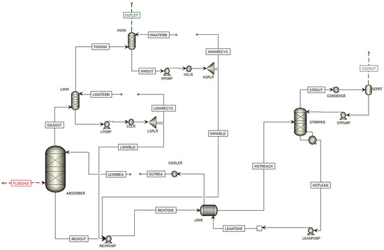
Figure 3. Simulation flowsheet of Scenario H14 in Aspen Plus.
Table 2 shows the summary of the key parameters in scenario H14 compared with the results of the simulation.
Table 2. Experimental data for scenario H14 compared with the simulation results.
The results show that the experimental and simulated numbers are close but not exactly the same.
4.1.2. Scenario F17, Faramarzi (2017)
Scenario F17 is data from the report published by Faramarzi [19]. This report was produced during the 2015 test campaign at TCM as a part of an independent verification protocol. Table 3 shows the summary of the key parameters in scenario F17 compared with the results of the simulation.
Table 3. Experimental data for scenario F17 compared with the simulation results.
Also, here, the results show that the experimental and simulated numbers are close but not exactly the same.
4.1.3. CHP Flue Gas Model Validation Results
The rate-based model with defined parameters and properties was simulated for the CHP flue gas at the TCM plant. The results show less than 4% deviation in CO2 removal efficiency, rich loading, stripper overhead, and bottom temperature. There is 3.6–8.5% derivation in the reboiler duty, produced CO2 flow rate, and SRD. Figure 4 shows the deviation between the experimental data and the simulation results for the important parameters in the validation of the model for CHP flue gas (scenario H14).
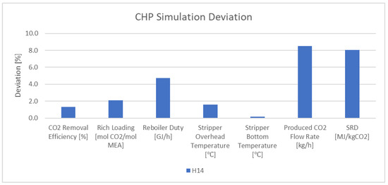
Figure 4. Deviation between the experimental data and the simulation results for CHP flue gas.
4.2. RFCC Flue Gas Simulation
Several validation tests for the rate-based model in Aspen Plus were also performed on the RFCC flue gas using the test campaigns’ performance data. However, the data from the test campaigns using RFCC flue gas are not as detailed as the results for the test campaigns using the CHP flue gas. The flowsheet of the simulated plant here is similar to the flowsheets for the CHP flue gas.
4.2.1. Scenario S21, Hume (2021)
Scenario S21 is data from the report published by Hume [23] during a test campaign at TCM in 2018.
In this simulation, RFCC flue gas is used in the simulation with only an 18 m absorber packing height. Only an RFCC stripper with no LVC configuration was used in this scenario. Table 4 shows the summary of the key parameters in scenario S21 compared with the results of the simulation.
Table 4. Experimental data for scenario S21 compared with the simulation results.
4.2.2. Scenario S6C, S6A, and S4, Ismail Shah (2019)
Scenarios S6C, S6A, and S4 are data from the report published by Shah et al. [20] during a test campaign at TCM in 2018. They used six different cases at the TCM plant, but only three of them are used in this study.
4.3. Rich Bypass Configuration Simulation
Scenarios Shah1, Shah2, Shah3, Shah4, and Shah5 are data from the report published by Shah et al. [6] during a test campaign at TCM. They used six different cases at the TCM plant, and in five of them, they used cold rich-solvent bypass to stripper overhead. Only the five cases with rich-solvent bypass configuration are used in this study. Moreover, the MEA data from the test campaigns in 2017 and 2018 (MEA-1 to MEA-5) were used in this campaign. Figure 5 shows the flowsheet of the simulated plant based on the test campaign in Aspen Plus.
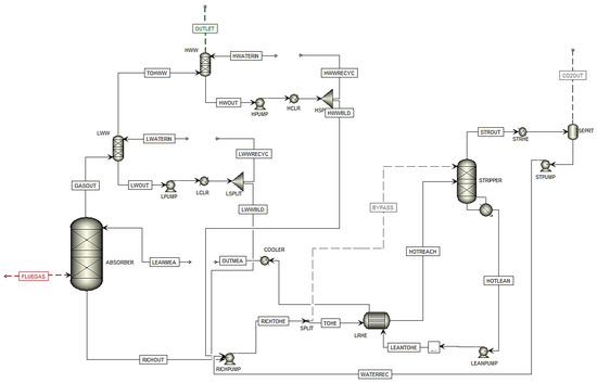
Figure 5. Simulation flowsheet of Ismail Shah test campaign (2021) in Aspen Plus.
RFCC Flue Gas Model Validation Results
The rate-based model with defined parameters and properties was simulated for the RFCC flue gas at the TCM plant. However, not many details in the experimental data are available in these test campaigns’ reports. The results show a relatively large deviation for scenarios M190 and M191 in both SRDs, which is 10.1–12.8%, and CO2 capture efficiency, which is 15.3–15.8%. In comparison with these scenarios, there is more consistency in the deviation of scenarios S21, S6C, S6A, and S4. The results show a less than 2% deviation in stripper bottom temperature and a less than 6% deviation in SRD. There is also a less than 5% deviation in CO2 capture efficiency for these scenarios. Figure 6 shows the deviation between the experimental data and the simulation results for the important parameters in the validation of the model for RFCC flue gas. Figure 6 shows the deviation between the experimental data and the simulation results for the important parameters in the validation of the model for CHP flue gas.
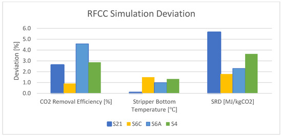
Figure 6. Deviation between the experimental data and the simulation results for RFCC flue gas.
5. TCM Plant Simulation and Optimization
This section presents the extended and verified rate-based model in Aspen Plus to simulate the TCM plant with a more detailed heat exchanger simulation. The limitations for each piece of installed equipment at the plant are discussed and obtained by the simulation. Moreover, a modification of the model to obtain the maximum capacity of the plant and an optimization of the operating condition and energy consumption for maximum CO2 removal efficiency are also presented in this section.
5.1. Designing the Real Heat Exchangers with Aspen EDR
To simulate and find the limitations of the real plant with all the equipment, a more detailed simulation is needed. All the heat exchangers in the Aspen Plus rate-based simulation are designed with Aspen Exchanger Design and Rating (Aspen EDR) v.12 in this section.
In Section 4, heat exchangers were simulated either in “design” mode in Aspen Plus or as a simple cooler or heater with a defined outlet temperature and pressure drop. Aspen EDR can simulate different types of heat exchangers based on real manufacturer data and calculate the outlet temperature and pressure of both cold and hot streams.
To change each of the coolers and heat exchangers in Aspen Plus to a real version, specific heat exchangers with the real manufacturer data and dimensions are defined in Aspen EDR with the imported process data from the previous Aspen Plus simulation. The process data should also include fouling resistance and the estimated and allowable pressure drop in each stream. The EDR simulation will present thermal, hydraulic, and mechanical results, as well as an API sheet, including the outlet process data, vapor and liquid properties, and the heat exchanger configuration. The EDR file can then be used as an input for Aspen Plus after changing the heat exchangers from “design” to “simulation” mode.
The heat exchangers at the TCM plant that must be replaced with the real model include a DCC cooler, water wash cooler, AIC cooler, lean/rich heat exchanger, lean cooler, condenser, and RFCC and CHP reboiler. The reboilers used in the strippers are designed internally and not by Aspen EDR. However, the simulation results and the limitations of the reboilers will be checked constantly by defining a pseudostream in the strippers.
5.2. Simulation Modifications
The necessary specifications in the simulations and the modification of the simulated plant are presented in this section. Different modifications and configurations discussed here are considered in all the further simulations on the TCM plant.
5.2.1. Process Flowsheet of the TCM Plant
Figure 6 shows the simulation flowsheet of the TCM plant simulated in Aspen Plus, which is shown in two separate parts: one for the DCC and the spray tower and one for other parts of the plant, including absorber, strippers, etc. (the total flowsheet of the plant is also shown in Appendix A).
As shown in Figure 7, advanced configurations at the TCM plant are used in the rate-based model simulation. A spray tower and DCC column are used to cool down the flue gas before entering the absorber. On top of the absorber column, the water wash system is simulated in two separate columns. An absorber intercooler (AIC) is also implemented in this simulation, which is marked by a blue dotted line.
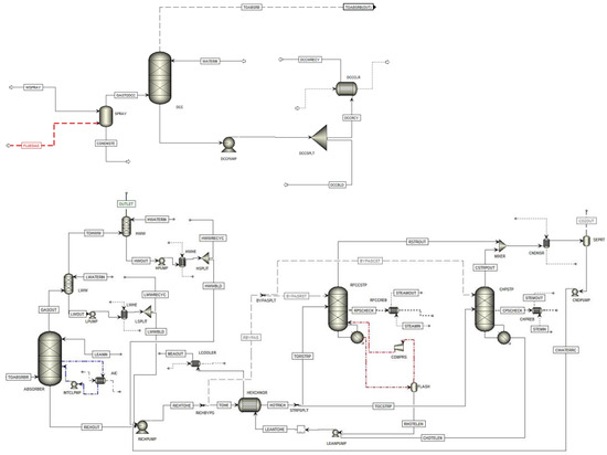
Figure 7. Simulation flowsheet of the TCM plant in Aspen Plus.
The RFCC and CHP strippers are simulated in two separate columns. A possible LVC configuration is also implemented in the RFCC stripper and is marked with a red dotted line. A condenser, a lean/rich heat exchanger, a lean cooler, and lean and rich pumps are also implemented in the model.
A cold rich-solvent bypass separator is marked with “RICHBYPS” before the lean/rich heat exchanger and sends the bypass flow to the strippers. The separator marked with “BYPASPLT” splits the bypass flow between RFCC and CHP strippers. The separator marked with “STRPSPLT” splits the hot-rich amine flow between the RFCC and CHP stripper. In general, the split fraction for “BYPASPLT” and “STRPSPLT” is the same amount.
5.2.2. Scenario MHP
Scenario MHP is used for the simulation of the TCM plant in this study. This is a Mongstad refinery flue gas from a gas-fired heat plant. This plant worked as a CHP plant previously, but now, the combustion energy is only used for heating without power production. The CO2 concentration of the gas is 10%, and the gas has a temperature of 145 °C and a pressure of 1.05 bar.
5.2.3. Parameters to Be Fixed
The main purpose of this TCM simulation model is to find the maximum plant operation capacity. As a result, the CO2 removal efficiency is fixed at 90% by adjusting the lean amine flow rate, and the gas flow rate is changed until the equipment limits at the plant are found. Amine lean loading is also fixed as 0.2 mol CO2/mol MEA in the simulations. The results of other important parameters, such as reboiler duty, SRD, and stripper bottom and top temperature, are observed and compared in the next sections.
5.2.4. Cold Rich-Solvent Bypass
A cold rich-solvent bypass before the lean/rich amine heat exchanger to the stripper top is implemented at the TCM plant and was considered in the modified simulation of the plant in this study. A default value of 20% for the bypass fraction was considered, and this value is varied. However, this amount can be modified based on the plant and stripper capacity, as in a previous study [6].
5.2.5. Temperature Adjustment of the Outlet Gas
The temperature of the gas going out of the top of the water wash system should be the same as the temperature of the gas going to the absorber to maintain the water balance in the plant. The reason is that temperature differences will create condensed water in the plant and can affect the calculations. In all TCM plant simulations, these temperatures should remain close, and this is performed by adjusting the water inlet flow rate of the heat exchangers in the water wash loops.
5.2.6. Other Considerations
- It is necessary to avoid flooding in the absorber and DCC column. As a result, in each simulation, the absorber hydraulic plot is monitored, so the flooding percentage (the approach to flooding) is not more than 70%. This amount is set by TCM as the warning limit for flooding;
- The outlet MEA of the lean cooler has the same temperature as the inlet MEA to the absorber. However, there is a pressure difference and a small difference in the flow rate of these two streams. This matter is not solved accurately in the simulations here, since it causes convergence problems, but at the TCM plant, it can be solved by using elevations before sending the lean amine from the lean cooler to the absorber;
- In addition to the rich-solvent bypass, a stripper separator is also implemented in the plant to be able to decide how much of the solvent should be directed to the CHP or RFCC stripper. There is the same amount of splitting percentage for the bypass flow to the strippers and the rich amine flow to the strippers, but it is not the same as the rich-solvent bypass fraction.
5.3. The Limitations of the TCM Plant
There are many limitations and bottlenecks at the TCM plant that can affect the operation by the maximum capacity. The most important limitations that must be considered in the simulations are found and listed in Table 5. Scenario MHP with only RFCC stripper is used in the simulations to find the limits for the absorber column. The RFCC stripper is larger than the CHP stripper, and it can process larger solvent amounts, and this is the reason that this stripper is used in the simulation.
Table 5. Absorber column limits at TCM plant by operating in the maximum flow capacity with scenario MHP.
5.3.1. Absorber Column Flooding Approach
The approach to flooding must also be less than 70% in the absorber column at all sections. The maximum possible inlet gas flow rate to the absorber while being in the flooding limit is found by the simulation to be 52,000 Sm3/h.
5.3.2. Reboiler Duty
There are limitations in the reboiler duty in the RFCC and CHP strippers at the TCM plant. The maximum possible reboiler duty for the RFCC stripper is 8.4 MW, and for the CHP stripper, 3.4 MW. New modifications should be considered in case of a higher need for reboiler duty in each stripper.
5.3.3. Real Capacity of the Reboilers
Even though the reboiler duty is within the defined limits of TCM, there is a possibility that the real reboilers at the TCM plant cannot operate properly at a very high flow rate. As a result, there is a need to check the performance of the real reboilers at specific flow rates in each simulation.
A pseudostream is added at stage 19 of each stripper with the real CHP and RFCC reboiler, designed in Aspen EDR, to check the performance of the real reboilers. The flow rate of the pseudostream should be the same as the total liquid flow at stage 19, observed in the stripper profile. The real reboiler duty is constantly checked in each simulation, and it must not be less than the defined reboiler duty in the stripper to be able to convey the required heat. The pseudostream and the simulated reboilers are shown in Figure 6 with black dotted lines.
5.3.4. The Capacity of the Heat Exchangers
Designing the real heat exchangers in Aspen EDR provides the possibility to check whether they can operate at the given flow rates or not. The Aspen Plus simulation will not show the results if the heat exchangers cannot convey the given flows.
5.3.5. Lean Amine Flow Rate
The lean amine flow rate entering the absorber column cannot exceed the maximum limit. This is due to the maximum possible amine velocity. At the TCM plant, there is a maximum allowable lean amine flow rate of 230 ton/h.
5.4. Plant Optimization for Maximum Gas Flow Rate
In the previous section, scenario MHP with only an RFCC stripper and a default bypass fraction value of 20% was used with the maximum possible flue gas to the absorber column. Moreover, the maximum allowable reboiler duty of 8.4 MW was used in the stripper. The lean amine loading of the lean cooler outlet in this configuration was 0.229 mol CO2/mol MEA, which is higher than 0.2 mol CO2/mol MEA in the inlet lean amine. As a result, the RFCC stripper alone cannot handle the total solvent and achieve the required stripping efficiency and lean loading. In this section, different configurations with scenario MHP are simulated to adjust the lean loading.
5.4.1. Cold Rich-Solvent Bypass Fraction Optimization
The amount of cold rich-solvent bypass fraction can affect the required reboiler duty and lean loading. As a result, an optimization study is performed on the same configuration used in the previous section, and the bypass fraction is changed between 0 and 30%. Figure 8 shows the optimization result of the rich-solvent bypass fraction.
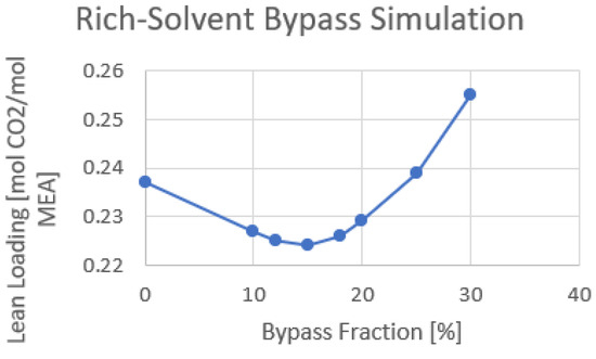
Figure 8. Cold rich-solvent bypass fraction optimization using only RFCC stripper.
A bypass fraction of 15% shows the minimum lean loading with 0.224 molCO2/molMEA out of the lean cooler. It is expected that the bypass fraction giving the lowest lean loading is close to the energy optimum bypass fraction.
5.4.2. Using Both CHP and RFCC Stripper
To operate within the practical conditions of the TCM plant, the maximum reboiler duty of the RFCC stripper cannot be more than 8.4 MW. As a result, a new modification of the simulation is performed to use both CHP and RFCC strippers at the same time with the maximum flow capacity.
In this simulation, the cold rich-solvent bypass remained at 15%, but the split fraction to the strippers and the reboiler duty of the strippers are adjusted to have the necessary splitting efficiency and the same outlet lean loading from both strippers and the outlet lean loading from the lean cooler as the inlet lean loading. Table 6 shows the modified parameters used in the RFCC and CHP strippers to adjust the lean loading.
Table 6. Modified parameters of RFCC and CHP strippers to adjust the lean loading.
This configuration allows one to use the maximum gas flow capacity, achieving 90% CO2 removal efficiency while operating at the practical limits of the TCM plant.
5.5. Plant Optimization for Maximum CO2 Removal Efficiency
TCM plant limitations to operate with the maximum gas flow capacity were found in the previous section, and the operation was modified considering the practical limitations. This section presents the maximum achievable CO2 removal efficiency at TCM by operating at the maximum plant capacity.
The CO2 removal efficiency is not fixed at 90% in this section, but the gas flow rate is fixed at the maximum operating limit for the absorber, and the amine flow rate is fixed at the maximum flow limit.
5.5.1. Maximum Achievable CO2 Removal Efficiency
To find the maximum achievable CO2 removal efficiency at the TCM plant using the maximum allowable flue gas flow rate, the amine flow rate needs to be increased. The maximum inlet amine flow rate is set to 230 ton/h, as mentioned before, and is used in this simulation.
A similar approach for the results of the lean loading is considered in this simulation, in which the outlet lean loading from both strippers must be the same as the outlet lean loading from the lean cooler and in the inlet amine solution. This amount is considered as 0.2 mol CO2/mol MEA.
Using the maximum allowable gas and amine flow rate will give a CO2 removal efficiency of 98% at the TCM plant. Table 7 shows the simulation parameters using the maximum capacity of the plant.
Table 7. Modified parameters of RFCC and CHP strippers with maximum CO2 removal efficiency.
5.5.2. Cold Rich-Solvent Bypass Optimization Using Maximum Capacity
As mentioned before, changing the rich amine flow rate to each of the strippers can affect the required reboiler duty. As a result, a new optimization on cold rich-solvent bypass using the maximum amine and gas flow rate at the TCM plant is performed. In this optimization, the flow fraction for strippers remains constant as in the previous simulation, and the cold rich-solvent bypass fraction is changed between 15 and 22%.
A minimum outlet amine lean loading, a minimum SRD, and a maximum produced CO2 flow rate are observed using 19% of the rich-solvent in bypass flow. The trend is shown in Figure 8. This means that the total reboiler duty used in the strippers can also be decreased. By adjusting the lean loading to 0.2 mol CO2/mol MEA, the reboiler duty for CHP and RFCC stripper is 8.4 and 2.17 MW, respectively. The total reboiler duty and SRD are 10.57 MW and 3.63 MJ/kg CO2, which is less than using 15% of the bypass fraction. This trend is shown in Figure 9.
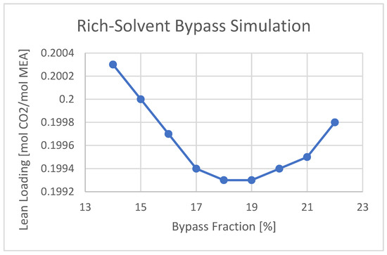
Figure 9. Cold rich-solvent bypass fraction optimization considering lean loading using maximum capacity.
6. Discussion
This section presents a discussion of the model accuracy, plant optimization, and energy consumption, as well as recommended future work.
6.1. Model Accuracy
The Aspen Plus rate-based model used in this study has been tested with many different scenarios, using different configurations and inlet flue gases, with several correlations available for mass transfer numbers, heat transfer numbers, interfacial area, and holdup [8]. This study aimed to check whether the model can show a reliable similarity between the experimental data from different test campaigns and the simulation results. As a result, no change has been made in the rate-based model parameters, such as the interfacial area factor or the liquid holdup factor. The only adjustments were to change the interfacial area, holdup, and mass and heat transfer method to gain the best possible results. There is still potential to adjust the model for more accurate simulation results or to predict the plant performance by changing parameters.
The results obtained from the model verification with different scenarios show that the model can provide more reliable data with more detailed input parameters for both flue gas and inlet lean amine to the absorber.
In one simulation, 98% CO2 removal was achieved with an SRD of 3.63 MJ/kg CO2 removed. This is a very good result, but it has some uncertainty. The reboiler temperature was especially higher than the normally recommended 120 °C, and the inlet CO2 concentration was especially high.
In this work, as in earlier works, a model has been validated by fitting it to performance data, and the model has been used to predict the effects of varying parameters. In the literature, a few successful attempts to predict performance in amine-based CO2 capture plants at conditions other than those measured have been published [5,7,20,28]. It is, in general, uncertain how accurate these predictions are without comparing them with performance data.
6.2. Cold Rich-Solvent Bypass Optimization for Minimum Energy Consumption
Having a rich-solvent bypass allows greater flashing of the CO2 from the hot rich-solvent stream and allows further release of CO2 in the upper stages of the stripper, which can increase the removal efficiency [5]. In this study, the cold rich-solvent bypass fraction was varied to find the minimum lean amine loading out of the stripper. A minimum in lean loading, and thus the reboiler duty and SRD, was found by a 15% split fraction, using only an RFCC stripper, and a 19% split fraction using both strippers and maximum amine flow rate.
To understand why the minimum in the reboiler duty and the amine lean loading occurs, we need to consider the energy provided by the reboiler. In addition to reversing the CO2 absorption reaction and increasing the amine temperature, the heat provided by the reboiler will generate steam in the column. The steam will lower the CO2 operating partial pressure below that of the equilibrium partial pressure, and thus, stripping occurs. With more flow as the split stream, a lower flow rate goes through the lean/rich heat exchanger. This means that the hot-rich amine will have a higher temperature and thus a higher vapor fraction, which leads to more steam generated for the pre-stripping process. The additional steam can have no benefit for the cold stream at the top of the stripper. As a result, a minimum in the reboiler duty should occur when a balance happens between the vapor generated in the reboiler and the energy needed by the cold rich-solvent for the pre-stripping process.
6.3. Energy Optimization
In addition to presenting the plant’s capacity and limitations, some modifications have been made for the energy optimization of the TCM plant. This includes the absorber, the stripper, and the condenser.
This study presents the optimum operation conditions of different configurations that can reduce the energy consumption in the plant. These conditions were presented based on the practical limitations of the heat exchangers, reboiler duties, absorber and DCC column, and lean amine flow rate.
By using the maximum plant capacity in amine flow and flue gas flow rate, the energy consumption of the plant is also increased. Using the same cold rich-solvent bypass fraction shows the total reboiler duty and SRD of 10.62 MW and 3.64 MJ/kgCO2, respectively. By using 19% as the bypass fraction, lower SRD and reboiler duty, together with higher CO2 production, are observed. The reason is that with a good balance between the vapor generated in the reboiler and the energy needed by the cold rich-solvent, more pre-stripping process happens, resulting in more CO2 production.
6.4. Future Work
Simulation of the TCM plant and finding different limitations and capacities have more potential. This study presented some, but not all, the aspects of the plant optimization process simulation. Some recommendations for future work on the TCM plant are presented below:
- The same procedure for this study can be performed on RFCC flue gas or other future scenarios provided by TCM. Finding the plant capacity and maximum achievable CO2 removal efficiency can also be performed using other operating scenarios;
- The simulation can be extended by using the maximum heat exchanger area in the plant. There are physical possibilities at TCM to use multiple or larger heat exchangers in each piece of equipment of the plant, and the operating capacities can vary in a new heat exchanger configuration;
- The stripper pressure in this study was considered as a constant amount between 1.85 and 1.95 bar. Using a high-pressure stripper is another possibility at the TCM plant. A thorough study of different stripper pressures and their effect on lean loading can be performed for future work. Moreover, operating under higher pressure and possible effects on the overall cost should be considered;
- In general, it is recommended to continue working with parallel modeling to optimize the operating conditions and run performance tests at TCM.
7. Conclusions
In this thesis, the CO2 capture process at Technology Centre Mongstad (TCM) using an MEA solution has been simulated using a rate-based model in Aspen Plus. The main purpose of this study was to develop a rigorous model for the TCM plant with modified configurations that generates reliable simulation results to be able to find the operating limits and maximum utilization capacity for each piece of installed equipment at TCM, as well as the optimum operation condition to achieve the maximum CO2 removal efficiency.
The rate-based model accuracy was tested using different scenarios based on the reports from test campaigns, and the simulation results of different configurations were presented. No change was made in the interfacial area factor or the liquid holdup factor, and the only adjustment was to change the interfacial area, holdup, and mass and heat transfer methods.
The model verification was performed with different scenarios and configurations, and the deviation between the experimental data and the simulation results for the process parameters were compared. This was performed in general with three main configurations, including CHP flue gas, RFCC flue gas, and cold rich-solvent bypass. CO2 removal efficiency is usually the most important parameter to be compared between the experimental and the simulation results. The deviation of the CO2 removal efficiency is less than 3% in all scenarios using CHP flue gas and less than 2.5% in rich-solvent bypass.
In general, there is better consistency between the experimental and simulation data with more detailed input parameters for flue gas and lean amine. However, some other parameters can affect the results, even though detailed data have been provided.
The results from this study show that the carbon capture process at TCM and the energy consumption at the plant can be optimized for the maximum plant capacity and considering the operation limits with a rigorous rate-based model.
Author Contributions
Conceptualization, S.H.K., K.R.P. and L.E.Ø.; methodology, S.H.K., K.R.P. and L.E.Ø.; software, S.H.K. and K.R.P.; validation, S.H.K., K.R.P. and L.E.Ø.; formal analysis, S.H.K., K.R.P. and L.E.Ø.; investigation, S.H.K. and L.E.Ø.; resources, S.H.K. and L.E.Ø.; data curation, S.H.K. and L.E.Ø.; writing—original draft preparation, S.H.K. and L.E.Ø.; writing—review and editing, S.H.K. and L.E.Ø.; visualization, S.H.K. and L.E.Ø.; supervision, K.R.P. and L.E.Ø.; project administration, S.H.K., K.R.P. and L.E.Ø. All authors have read and agreed to the published version of the manuscript.
Appendix A
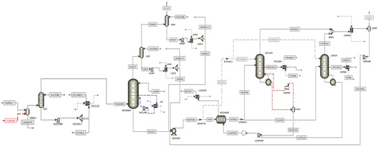
Figure A1. Simulation flowsheet of TCM plant.
References
- Technology Centre Mongstad|Test Centre for CO2 Capture. Available online: https://tcmda.com/about-tcm/ (accessed on 3 May 2023).
- Li, B.; Duan, Y.; Luebke, D.; Morreale, B. Advances in CO2 capture technology: A patent review. Appl. Energy 2013, 102, 1439–1447. [Google Scholar] [CrossRef]
- Øi, L.E.; Eldrup, N.; Aromada, S.; Haukås, A.; Hæstad, J.H.; Lande, A.M. Process Simulation, Cost Estimation and Optimization of CO2 Capture using Aspen HYSYS. In Proceedings of the SIMS Conference on Simulation and Modelling SIMS 2020, Virtual Conference, 22–24 September 2020; pp. 326–331. [Google Scholar] [CrossRef]
- Aromada, S.A.; Øi, L.E. Energy and Economic Analysis of Improved Absorption Configurations for CO2 Capture. Energy Procedia 2017, 114, 1342–1351. [Google Scholar] [CrossRef]
- Arshad, N.; Alhajaj, A. Process synthesis for amine-based CO2 capture from combined cycle gas turbine power plant. Energy 2023, 274, 127391. [Google Scholar] [CrossRef]
- Shah, M.I.; Silva, E.; Gjernes, E.; Åsen, K.I. Cost Reduction Study for MEA based CCGT Post-Combustion CO2 Capture at Technology Center Mongstad. In Proceedings of the 15th Greenhouse Gas Control Technologies Conference, Abu Dhabi, United Arab Emirates, 15–18 March 2021. [Google Scholar] [CrossRef]
- Luo, X.; Knudsen, J.; de Montigny, D.; Sanpasertparnich, T.; Idem, R.; Gelowitz, D.; Notz, R.; Hoch, S.; Hasse, H.; Lemaire, E.; et al. Comparison and validation of simulation codes against sixteen sets of data from four different pilot plants. Energy Procedia 2009, 1, 1249–1256. [Google Scholar] [CrossRef]
- Zhang, Y.; Chen, H.; Chen, C.-C.; Plaza, J.M.; Dugas, R.; Rochelle, G.T. Rate-Based Process Modeling Study of CO2 Capture with Aqueous Monoethanolamine Solution. Ind. Eng. Chem. Res. 2009, 48, 9233–9246. [Google Scholar] [CrossRef]
- Experimental Validation of a Rigorous Absorber Model for CO2 Postcombustion Capture. SINTEF. Available online: https://www.sintef.no/en/publications/publication/371103/ (accessed on 6 February 2023).
- Zhang, Y.; Chen, C.-C. Modeling CO2 Absorption and Desorption by Aqueous Monoethanolamine Solution with Aspen Rate-based Model. Energy Procedia 2013, 37, 1584–1596. [Google Scholar] [CrossRef]
- Erikøi, L. Comparison of Aspen HYSYS and Aspen Plus simulation of CO2 Absorption into MEA from Atmospheric Gas. Energy Procedia 2012, 23, 360–369. [Google Scholar] [CrossRef]
- Cousins, A.; Wardhaugh, L.T.; Feron, P.H. Preliminary analysis of process flow sheet modifications for energy efficient CO2 capture from flue gases using chemical absorption. Chem. Eng. Res. Des. 2011, 89, 1237–1251. [Google Scholar] [CrossRef]
- Kvam, S.H.P. Vapor Recompression in Absorption and Desorption Process for CO2 Capture. Master’s Thesis, Høgskolen i Telemark, Porsgrunn, Norway, 2013. Available online: https://openarchive.usn.no/usn-xmlui/handle/11250/2439010 (accessed on 6 February 2023).
- Aromada, S.A.; Øi, L. Simulation of improved absorption configurations for CO2 capture. In Proceedings of the 56th Conference on Simulation and Modelling, Linköping, Sweden, 7–9 October 2015. [Google Scholar] [CrossRef]
- Rehan, M.; Rahmanian, N.; Hyatt, X.; Peletiri, S.P.; Nizami, A.-S. Energy Savings in CO2 Capture System through Intercooling Mechanism. Energy Procedia 2017, 142, 3683. [Google Scholar] [CrossRef]
- Thimsen, D.; Maxson, A.; Smith, V.; Cents, T.; Falk-Pedersen, O.; Gorset, O.; Hamborg, E.S. Results from MEA testing at the CO2 Technology Centre Mongstad. Part I: Post-Combustion CO2 capture testing methodology. Energy Procedia 2014, 63, 5938–5958. [Google Scholar] [CrossRef]
- Chhaganlal, M.; Fostås, B.; Hamborg, E. Results from MEA testing at the CO2 Technology Centre Mongstad. Part II: Verification of baseline results. Energy Procedia 2014, 63, 5994–6011. [Google Scholar]
- Gjernes, E.; Pedersen, S.; Cents, T.; Watson, G.; Fostås, B.F.; Shah, M.I.; Lombardo, G.; Desvignes, C.; Flø, N.E.; Morken, A.K.; et al. Results from 30 wt% MEA Performance Testing at the CO2 Technology Centre Mongstad. Energy Procedia 2017, 114, 1146–1157. [Google Scholar] [CrossRef]
- Faramarzi, L.; Thimsen, D.; Hume, S.; Maxon, A.; Watson, G.; Pedersen, S.; Gjernes, E.; Fostås, B.F.; Lombardo, G.; Cents, T.; et al. Results from MEA Testing at the CO2 Technology Centre Mongstad: Verification of Baseline Results in 2015. Energy Procedia 2017, 114, 1128–1145. [Google Scholar] [CrossRef]
- Shah, M.I.; Lombardo, G.; Fostås, B.; Benquet, C.; Kolstad Morken, A.; de Cazenove, T. CO2 Capture from RFCC Flue Gas with 30w% MEA at Technology Centre Mongstad, Process Optimization and Performance Comparison. In Proceedings of the 14th Greenhouse Gas Control Technologies Conference Melbourne, Melbourne, Australia, 21–25 October 2018. [Google Scholar] [CrossRef]
- Meuleman, E.; Awtry, A.; Silverman, T.; Heldal, S.; Staab, G.; Kupfer, R.; Panaccione, C.; Brown, R.; Atcheson, J.; Brown, A.E. ION 6-Month Campaign at TCM with its Low-Aqueous Capture Solvent Removing CO2 from Natural Gas Fired and Residue Fluid Catalytic Cracker Flue Gases. In Proceedings of the 14th Greenhouse Gas Control Technologies Conference Melbourne, Melbourne, Australia, 21–25 October 2018. [Google Scholar] [CrossRef]
- Fosbøl, P.L.; Neerup, R.; Almeida, S.; Rezazadeh, A.; Gaspar, J.; Knarvik, A.B.N.; Flø, N.E. Results of the fourth Technology Centre Mongstad campaign: LVC testing. Int. J. Greenh. Gas Control. 2019, 89, 52–64. [Google Scholar] [CrossRef]
- Hume, S.; Shah, M.I.; Lombardo, G.; de Cazenove, T.; Feste, J.K.; Maxson, A.; Benquet, C. Results from MEA Testing at the CO2 Technology Centre Mongstad. Verification of Residual Fluid Catalytic Cracker (RFCC) Baseline Results. In Proceedings of the 15th Greenhouse Gas Control Technologies Conference, Abu Dhabi, United Arab Emirates, 15–18 March 2021. [Google Scholar] [CrossRef]
- Larsen, I.S. Simulation and Validation of CO2 Mass Transfer Processes in Aqueous MES Solution with Aspen Plus at CO2 Technology Centre Mongstad. Master’s Thesis, Faculty of Technology, Telemark University College, Porsgrunn, Norway, 2014. [Google Scholar]
- Desvignes, C. Simulation of Post-Combustion CO2 Capture Process with Amines at CO2 Technology Centre Mongstad. Master’s Thesis, CPE Lyon, Villeurbanne, France, 2015. [Google Scholar]
- Zhu, Y. Simulation of CO2 Capture at Mongstad Using Aspen HYSYS. Master’s Thesis, Faculty of Technology, Telemark University College, Porsgrunn, Norway, 2015. [Google Scholar]
- Sætre, K.A. Evaluation of Process Simulation Tools at TCM. Master’s Thesis, Faculty of Technology, University College of Southeastern Norway, Porsgrunn, Norway, 2016. [Google Scholar]
- Øi, L.E.; Sætre, K.A.; Hamborg, E.S. Comparison of simulation tools to fit and predict performance data of CO2 absorption into monoethanol amine at CO2 Technology Centre Mongstad (TCM). In Proceedings of the 59th Conference on Imulation and Modelling (SIMS 59), Oslo Metropolitan, Norway, 26–28 September 2018; pp. 230–235. [Google Scholar] [CrossRef]
- Fagerheim, S. Process Simulation of CO2 Absorption at TCM Mongstad. Master’s Thesis, University of South-Eastern Norway, Notodden, Norway, 2019. Available online: https://openarchive.usn.no/usn-xmlui/handle/11250/2644680 (accessed on 30 January 2023).
- Sæter, N. Process Simulation of CO2 Absorption Data Fitted to Performance Efficiency at TCM Mongstad. Master’s Thesis, Faculty of Technology, Natural Sciences, and Maritime Science, University of South-Eastern Norway, Porsgrunn, Norway, 2021. [Google Scholar]
- Montañés, R.M. Transient Performance of Combined Cycle Power Plant with Absorption Based Post-Combustion CO2 Capture: Dynamic Simulations and Pilot Plant Testing. Doctoral Thesis, NTNU, Trondheim, Norway, 2018. Available online: https://ntnuopen.ntnu.no/ntnu-xmlui/handle/11250/2506461 (accessed on 4 July 2024).
- Bui, M.; Flø, N.E.; de Cazenove, T.; Mac Dowell, N. Demonstrating flexible operation of the Technology Centre Mongstad (TCM) CO2 capture plant. Int. J. Greenh. Gas Control. 2020, 93, 102879. [Google Scholar] [CrossRef]
- Putta, K.R.; Saldana, D.; Campbell, M.; Shah, M.I. Development of CO2 Capture Process Cost Baseline for 555 MWe NGCC Power Plant Using Standard MEA Solution. In Proceedings of the 16th Greenhouse Gas Control Technologies Conference, Lyon, France, 23–27 October 2022. [Google Scholar] [CrossRef]
- Bravo, J.; Rocha, J.A.; Fair, J. Mass Transfer in Gauze Packings. Hydrocarbon Processing. 1985. Available online: https://www.semanticscholar.org/paper/Mass-transfer-in-gauze-packings-Bravo-Rocha/fbef768ce559366f045d9122cf39946f738b1186 (accessed on 4 July 2024).
- Bravo, J.; Rocha, J.A.; Fair, J. A comprehensive Model in the Performance of Columns Containing Structured packings, Distillation and Absorption. In Institution of Chemical Engineers Symposium Series; Hemsphere Publishing Corporation: London, UK, 1992; Volume 128. [Google Scholar]