
2. CESAR1 Solvent Degradation in Pilot and Laboratory Scale (2024)
Vanja Buvika*, Andreas Grimstvedta, Kai Vernstada, Merete Wiiga, Hanna K. Knuutilab, Muhammad Zeeshanc, Sundus Akhterc, Karen K. Høisæterc, Fred Rugenyic, Matthew Campbellc
*Corresponding author. Email address: vanja.buvik@sintef.no
aSINTEF Industry, NO-7465 Trondheim, Norway
bDepartment of Chemical Engineering, Norwegian University of Science and Technology (NTNU), N-7497- Trondheim, Norway
cTechnology Centre Mongstad, NO-5954 Mongstad, Norway

Abstract
A CESAR1 solvent sample which had been subjected to a series of test campaigns with industrial flue gases was analysed for identified degradation compounds with newly developed analytical techniques. Before analysing the pilot sample, the degradation compounds of CESAR1 were identified in samples from laboratory scale oxidative and thermal degradation stress tests with aqueous 2-amino-2-methyl-propanol (AMP), piperazine (PZ) and the CESAR1 blend. Three new major degradation compounds, which have previously not been identified, were found among the ten most abundant degradation species. A total of 35 degradation compounds were found in the solvent sample, whereof 12 have not been previously identified neither in CESAR1 nor during degradation of AMP or PZ alone. By comparing the quantified solvent amines and degradation compounds with the total concentration of nitrogen in the sample, it was found that all major nitrogen containing degradation compounds are accounted for, and that the nitrogen containing species in the solvent have been identified and quantified within the analytical uncertainty. This contributes to closing one of the major knowledge gaps associated with CO2 capture operations with the CESAR1 solvent, which is a target of the Horizon Europe project AURORA.
Keywords: AMP, piperazine, stability, oxidative and thermal degradation
1. Introduction
The non-proprietary CESAR1 amine blend has been widely studied for use as a solvent for post-combustion CO2 capture (Campbell et al., 2022; Knudsen et al., 2011; Mangalapally and Hasse, 2011; Moser et al., 2023; Rabensteiner et al., 2016). Despite of its relative popularity in the solvent market, there are still many knowledge gaps connected to the stability of CESAR1 (Morlando et al., 2024). The mixture of 2-amino-2-methyl propanol (AMP, CAS 124-68-5) and piperazine (PZ, CAS 110-85-0) is known to be much more stable than ethanolamine (MEA, CAS 141-43-5), both under oxidising conditions, thermal stress, and at the cyclic conditions in the CO2 capture plant.
Even though the stability of CESAR1 is higher compared to other solvents, the degradation phenomena still need to be fully understood before the solvent can be safely implemented for large or full-scale CO2 capture from industrial sources. Amine solvents degrade due to reactions between the amine and reactive species present in the flue gas (such as O2, SOX and NOX.), high temperatures and presence of catalytic amounts of dissolved metals (Buvik et al., 2021; Dumée et al., 2012; Flø et al., 2017; Vega et al., 2020). The degradation can lead to reduced process efficiency, high solvent replacement and reclaiming costs, as well as corrosion or fouling of the construction materials. If the degradation compounds that form are more volatile than the solvent amine(s), it can also lead to increased emissions into the atmosphere where they can impact the environment. Understanding solvent degradation is therefore important from both environmental, economic, and safety perspectives.
All amines produce some generic degradation products, like carboxylates (i.e., formate, acetate, etc.), aldehydes (formaldehyde, acetaldehyde), and ammonia (Vevelstad et al., 2022). Additionally, they will produce solvent specific compounds, which will depend on the chemical structure of the amine in use. For CESAR1, although many potential degradation products have been suggested in the literature, especially through studies on AMP and PZ (Eide-Haugmo et al., 2011; Freeman et al., 2010; Freeman and Rochelle, 2012; Lepaumier et al., 2009; Wang and Jens, 2014, 2012), only a limited number of degradation compounds were previously known. A thorough review of identified and suggested degradation compounds of AMP, PZ and their blends can be found in Morlando et al. (2024).
Despite of solvent degradation being low compared to other solvents, degradation phenomena need to be fully understood before a solvent can be safely implemented for large or full-scale CO2 capture from industrial sources, to fully comprehend potential environmental and operational impacts, and ensure safety for operators and neighbouring community. Therefore, this study aims to fully characterise the degraded CESAR1 solvent, to identify all the remaining compounds. To achieve this, analysis of the total (molar) concentration of nitrogen in the solvent is compared to the total (molar) concentration of nitrogen in known compounds, meaning the sum of nitrogen in AMP, PZ, known contaminants and degradation compounds. The literature has previously stated that about 50% of the nitrogen containing degradation compounds in AMP and PZ remain unidentified (Wang, 2013; Wang and Jens, 2014).
2. Materials and methods
2.1 Pilot samples
In the period from late 2019 to the end of 2020, Technology Centre Mongstad (TCM) ran multiple test campaigns to study the behaviour of the CESAR1 solvent at their post-combustion CO2 capture plant. These included the ALIGN CCUS CESAR1 campaign and two CESAR1 campaigns by the TCM owners (Benquet et al., 2021; Bui et al., 2022; Campbell et al., 2022; Drageset et al., 2022; Hume et al., 2021; Languille et al., 2021a, 2021b). During these campaigns that were conducted successively at TCM, the solvent was subjected to both combined heat and power (CHP) flue gas and residue fluid catalytic cracking (RFCC) flue gas. In addition, two rounds of thermal reclaiming were conducted, and make-up solvent was added when needed. Altogether, the solvent sample studied in this work was in use in the TCM plant for about 13 months in total, and the analysed sample was taken after the plant was drained.
2.2 Oxidative and thermal degradation experiments
To get a more detailed understanding of the degradation seen at the pilot scale, some laboratory experiments were performed. In those experiments, AMP and PZ with purity of 99% was used to prepare the aqueous solutions of 3.0 mol/kg AMP, 1.5 mol/kg PZ, and the CESAR1 blend (3.0 mol/kg AMP + 1.5 mol/kg PZ). The solutions were gravimetrically preloaded with pure CO2 to the desired loading and analysed for amine and CO2 content to ensure correct loading before use in the experiments.
Oxidative degradation of the single amines and CESAR1 blend was performed according to Vevelstad et al. (2016) in a water bath heated double-jacketed glass reactor at 60 °C with 50 L/min of gas bubbled through the solution and circulated back to the solution. The solvent, pre-loaded with CO2 to contain 0.4 mol CO22 per mol amine functionality was used in the experiments. A catalytic amount of iron sulphate heptahydrate (FeSO4‧7H2O, 0.5 mmol/L) was added to the solvent. A small amount of gas (77% N2, 21% O2, 2% CO2) was continuously added to the reactor to ensure constant O2 concentration. A bleed leaving the reactor was taken through two double-jacketed condensers before exiting through two impinger bottles containing 0.1 M H2SO4 (aq.). Liquid samples were taken regularly, and a 2,4-dinitrophenylhydrazine (DNPH) cartridge was attached between the second condenser and the first impinger bottle for the last 4 days of the experiment.
Testing of the thermal stability of AMP, PZ and CESAR1 was performed in closed SS316L cylinders according to Lepaumier et al. (2011) over a period of 28 days, and some cylinders were withdrawn regularly for analyses. The temperature of 135 °C was used in all experiments and the solutions were loaded up to 0.4 mol CO2 per mol amine functionality.
2.3 Analytical methods
SINTEF evaluated nearly 100 potential degradation compounds. The basis for the evaluation was compounds proposed for AMP, PZ and their blends in the existing literature (Morlando et al., 2024) and analogous degradation mechanisms known for amines other than the CESAR1 components (Vevelstad et al., 2022). Compounds to analyse were selected based on their likelihood of formation and the possibility of obtaining analytical standards for method development. SINTEF already had analytical methods for many compounds. For others, SINTEF purchased analytical standards and developed LCMS quantification methods. The main goal was to be able to close the nitrogen balance of degraded CESAR1 samples. The LC-MS/MS methods used in this work are based on the same principles as those described in Vevelstad et al. (2023). An overview of compounds analysed using LC-MS/MS in the degraded solvent samples is given in Table 1.
Table 1: Compounds analysed in the degraded solvent samples.
| Abbrev. | Name | CAS-number |
| AAc | Acetic acid | 64-19-7 |
| – | Acetaldehyde | 75-07-0 |
| – | Acetone | 67-64-1 |
| AAEA | 2-amino-N-(2-aminoethyl)-acetamide | 84354-31-4 |
| AEAAC | N-(2-aminoethyl)-glycine | 24123-14-6 |
| AEAEPZ | 1-[2-(1-piperazinyl) ethyl]-1,2-ethanediamine | 24028-46-4 |
| AEAEPZ urea | 1-[2-(1-piperazinyl) ethyl]-2-imidazolidinone | 104087-61-8 |
| AEHA | N-(2-aminoethyl)-2-hydroxy- acetamide | 83019-76-5 |
| AEI | 1-(2-aminoethyl)-2-imidazolidone | 6281-42-1 |
| AIBA | 2-Aminoisobutyric acid | 62-57-7 |
| AMPAMP | 2-[(2-amino-2-methylpropyl)amino]-2-methyl-1-propanol | 72622-74-3 |
| AMP-NO2 | 2-methyl-2-(nitroamino)-1-propanol | 1239666-60-4 |
| AMPPZ | 2-amino-2-methyl-1-(1-piperazinyl)-1-propanone | 479065-33-3 |
| AMP urea | N,N‘-bis(2-hydroxy-1,1-dimethylethyl)-urea | 162748-76-7 |
| DAEP | 1,4-piperazinediethanamine | 6531-38-0 |
| DEA | Diethylamine | 109-89-7 |
| DFP | 1,4-piperazinedicarboxaldehyde | 4164-39-0 |
| DMA | dimethylamine | 124-40-3 |
| DMHTBI | 4,4-dimethyl-1-hydroxytertbutyl-2-imidazolidinone | 2761991-15-3 |
| DMOZD | 4,4-dimethyl-2-oxazolidinone | 26654-39-7 |
| DMP | 1,4-dimethylpiperazine | 160-58-1 |
| DM-PZEA | α,α-dimethyl-1-piperazineethanamine | 1259927-55-3 |
| DNPZ | N,N’-dinitrosopiperazine | 140-79-4 |
| DPA | Dipropylamine | 142-84-7 |
| EA | Ethylamine | 75-04-7 |
| EDA | Ethylenediamine | 107-15-3 |
| EMA | Ethylmethylamine | 624-78-2 |
| EPZ | 1-ethylpiperazine | 5308-25-8 |
| F-AMP | N-(2-hydroxy-1,1-dimethylethyl)formamide | 682-85-9 |
| FAc | Formic acid | 64-18-6 |
| – | Formaldehyde | 50-00-0 |
| FPZ | 1-piperazinecarboxaldehyde | 7755-92-2 |
| GAc | Glycolic acid | 79-14-1 |
| HEP | 1-piperazineethanol | 103-76-4 |
| HMeGly | N-(2-hydroxy-1,1-dimethylethyl)-Glycine | 1154902-47-2 |
| HPAc | 3-hydroxypropanoic acid | 503-66-2 |
| HTBI | 1-(1-Hydroxy-2-methylpropan-2-yl)imidazolidin-2-one | 1566510-82-4 |
| iBAc | Isobutyric acid | 79-31-2 |
| LAc | Lactic acid | 50-21-5 |
| MA | methylamine | 74-89-5 |
| MAMP | 2-methyl-2-(methylamino)-1-propanol | 27646-80-6 |
| MNPZ | N-nitrosopiperazine | 5632-47-3 |
| MPZ | 1-methylpiperazine | 109-01-3 |
| NMAMP | nitroso-N-methyl-2-amino-2-methylpropanol | 27646-81-7 |
| – | Ammonia | 7664-41-7 |
| OPZ | Piperazinone | 5625-67-2 |
| PA | Propylamine | 107-10-8 |
| PAc | Propionic acid | 79-09-4 |
| PEP | 1,1′-(1,2-ethanediyl)bis-piperazine | 19479-83-5 |
| PZ-NO2 | 1-nitropiperazine | 42499-41-2 |
| TMOX | 3,4,4-trimethyl-2-oxazolidinone | 15833-17-7 |
Analysis of total CO2 and total nitrogen (TN) concentration in the samples were performed on a Shimadzu TOC-LCPH with a TNM-L unit by SINTEF. Both systems were calibrated prior to use with NaHCO3 and ethanolamine, respectively.
3. Results and discussion
3.1 CESAR1 degradation compounds in the pilot sample
During the 2019 ALIGN CCUS campaign at TCM, samples were sent to SINTEF for quantification of selected and known degradation products at the time. These included 2,4-lutidine, 4,4-dimethyl-2-oxazolidione (DMOZD), N-methylpiperazine (MNPZ), 2-oxopiperazine (OPZ), formic acid (FAc), oxalic acid, glycolic acid (GAc), and propionic acid (PAc) (Benquet et al., 2021). Detailed results from this campaign have been described by Campbell et al. (2022). In this previous work, the total alkalinity was used to assess the state of the solvent. The observed results showed a deviation between the sum of known alkaline components in the sample and the measured total alkalinity, indicating the presence of unknown degradation products. Due to this, a sample from the end of the operation at TCM was characterized using the newly developed LC-MS/MS methods. The methods were used to analyse new degradation components in addition to the components analysed in the past. This work presents the results from the analysis of the sample from the end of operation of the 2019-2020 CESAR1 campaigns. It is important to note that, as the sample in question has been through multiple campaigns with different flue gas sources, including solvent make-up and thermal reclaiming, the ratio of the different degradation products is not necessarily representative of what would be found in a campaign solvent under normal operating conditions. It will, however, show which compounds can be expected to be seen under operation with CESAR1, and hence, contribute to closing knowledge gaps associated with CESAR1 degradation.
EDA, HMeGly, and TMOX were the most abundant degradation products found in the end of operations sample. Out of these three, HMeGly and TMOX have not previously been quantified in AMP, PZ, nor CESAR1 in the open literature. Figure 1 shows all the 33 components quantified in the sample from end of operation. Out of these 33 compounds, 11 AMP, PZ, or CESAR1-specific compounds have previously not been quantified. These include HMeGly, TMOX, DM-PZEA, AMPAMP, AMP-urea, AAEA, F-AMP, AIBA, AEHA, AEAEPZ, and PEP. Some additional generic degradation compounds that have also not been specifically reported to be found in CESAR1, namely HPAc, LAc, and EA were also found, as well as traces of two additional CESAR1-speficic compounds, AEAEPZ-urea and AMP-NO2. An additional 15 compounds not presented in the figure were below the quantitation limits of the methods used.
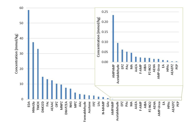
Figure 1: Concentrations of degradation compounds in CESAR1 solvent after ended operation at TCM.
When assessing the nitrogen balance, the total alkalinity only captures basic nitrogen-containing compounds which are partly neutralised by acidic components in the solvent (Waite et al., 2013). The total nitrogen provides a better assessment of the mass balance as it is not prone to the mentioned drawbacks. Total nitrogen (TN) analysis indiscriminately quantifies all nitrogen bound in any species (besides N2).
By adding up the nitrogen in all measured compounds and comparing this with the amount total nitrogen from the TN analysis, the contribution of the degradation products and the solvent amines to the nitrogen balance of the solvent can be assessed. Figure 2 shows that about 99% of the nitrogen in the solvent was accounted for. The solvent amines, AMP and PZ, account for 92% of the TN, while the quantified degradation products account for about 7% of the
nitrogen. Of these 7%, MAMP, which is a common contaminant in AMP found in the CESAR1 solvent before flue gas contact, accounted for around 1% of the TN. The degradation products which could be quantified by the previously available analytical methods, MNPZ, OPZ, and DMOZD, account for about 1%. Finally, the new degradation products presented in this work account for approximately 5% of the TN. The nitrogen balance closure from the newly identified and quantified degradation compounds underlines the value derived from the newly identified compounds and developed analytical methods in providing further insights into the behaviour of CESAR1. The analytical uncertainty of the TN analysis is ±10%, while that of each individual component is ±5%, making the 1% of nitrogen that is not accounted for insignificant. This does not mean that all degradation compounds of CESAR1 have been identified to date but indicates that all major nitrogen containing compounds are accounted for in this study.
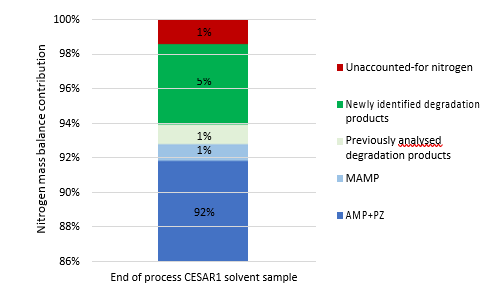
Figure 2: Summary of the nitrogen balance showing the contribution of AMP and PZ, previously quantified degradation products, newly identified degradation products and the unaccounted-for nitrogen. The unaccounted-for nitrogen could be due to uncertainties in the analytical methods used, unidentified degradation products or degradation compounds in concentrations below the limit of quantification of the measurement methods used or combinations thereof.
3.2 Comparison of the pilot samples to oxidative and thermal degraded AMP, PZ and CESAR1 blend
In the lab experiments, conditions that accelerate thermal or oxidative degradation are used. This allows relatively short experimental time and often leads to a degree of degradation that is not industrially acceptable, nor realistic. However, the advantage of these tests is that it is often easier to identify and analyse new degradation compounds as they are present in higher concentrations, and one can potentially find compounds that might otherwise only occur in quantifiable amounts after long-term operation. Furthermore, these laboratory scale tests allow for the identification of:
1) The conditions under which a compound forms (oxidative or thermal degradation), and
2) From which amines (PZ, AMP or both) they originate.
The main degradation compound (molar basis) of CESAR1 is EDA, which is a known oxidation product of PZ (Freeman et al., 2010). HMeGly is an amino acid that has not previously been identified or quantified in CESAR1, PZ or AMP. The laboratory experiments show that HMeGly is primarily formed during oxidative degradation of CESAR1, although some HMeGly is also formed in the thermal degradation experiments (maximum 5 mmol/kg). The concentration of HMeGly over time during oxidative degradation is shown in Figure 3a. The formation mechanism of HMeGly is likely to be analogous to that of N-(2-hydroxyethyl)-glycine (“HEGly”, CAS 5835−28-9) which is a major degradation compounds of MEA. Many reaction pathways for the formation of HEGly have been suggested (Vevelstad et al., 2016), without a clear consensus on which pathway is the most probable. HMeGly is likely to form through the same mechanism as HEGly in MEA, only with AMP as the reactant as opposed to MEA.
DM-PZEA is clearly a thermal degradation product that can only form in the blend of PZ and AMP, and not in each solvent separately. The concentration of DM-PZEA after 4 weeks of thermal degradation at 135°C in stainless steel cylinders is shown in Figure 3b. Oxidative degradation of CESAR1 gave a maximum DM-PZEA concentration of 4 mmol/kg after 6 weeks, while AMP and PZ alone never formed any DM-PZEA.
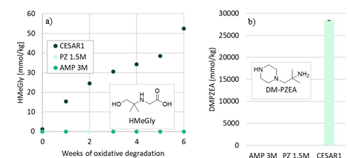
Figure 3: (a) Concentration of HMeGly during oxidative degradation experiments over time, and (b) concentration of DM-PZEA after thermal degradation at 135C in the presence of 0.4 mol CO2 per mol N.
DM-PZEA is suggested to form through a carbamate polymerisation type reaction, where the cyclic carbamate DMOZD reacts with PZ in a condensation reaction to form the “dimer” DM-PZEA, as shown in Figure 4. This degradation product was suggested by Li et al. (2013).
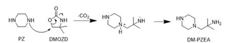
Figure 4: Suggested mechanism of formation of DM-PZEA.
TMOX is mainly a product of thermal MAMP degradation, and as MAMP is a common contaminant in technical AMP, TMOX can form during AMP and CESAR1 degradation as shown in Figure 5a. TMOX also forms to a lesser extent during oxidative AMP degradation, but is not present in significant amounts during oxidative degradation of the CESAR1 blend, as can be seen in Figure 5b. TMOX is hypothesised to form according to the mechanism described in Figure 6, by intramolecular condensation of the MAMP carbamate.
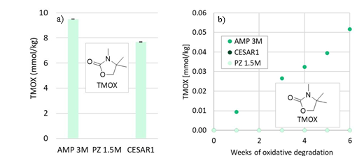
Figure 5: TMOX concentration (a) after thermal degradation at 135°C in the presence of 0.4 mol CO2 per mol N, and (b) during oxidative degradation.
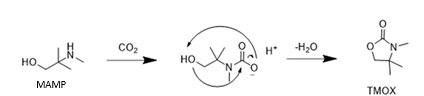
Figure 6: Suggested formation pathways of TMOX, analogously to that of DMOZD from AMP.
Another amino acid that is formed during CESAR1 degradation is AEAAC, which has been suggested to be a PZ degradation product in the literature (Freeman, 2011; Wang, 2013). This compound is likely formed through the same degradation mechanism as HMeGly and HEGly, where EDA is a likely reactant. The formation of AEAAC during laboratory scale oxidative degradation experiments is depicted in Figure 7a.
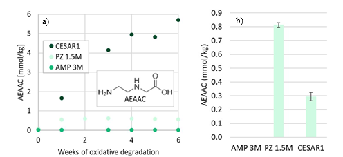
Figure 7: Concentration of AEAAC during (a) oxidative degradation experiments over time, and (b) after 4 weeks thermal degradation at 135°C with 0.4 mol CO2 per mol N.
Furthermore, DMOZD and AMPAMP are products of thermal AMP degradation. The oxidation products of PZ, OPZ and FPZ, form only in low concentrations during oxidative degradation of only PZ. Their formation rates, however, are greatly accelerated in the CESAR1 blend. MPZ and EPZ are thermal degradation products of PZ. Generally, all degradation reactions are accelerated in the CESAR1 blend compared to in the single amine 1.5M PZ or 3M AMP solvents. Despite the formation pathways in theory only requiring one of the species, the blend enhances formation in all cases except for the formation of AEAAC at thermally degrading conditions, shown in Figure 7b, in which case
more AEAAC was formed in PZ than in CESAR1. This can possibly be explained by the presence of competing reactants, i.e. AMP forming HMeGly with the same reactants as form AEAAC, and the HMeGly reaction having a lower activation energy.
4. Conclusions
In this work, 35 different degradation compounds were successfully identified and quantified in the degraded CESAR1 solvent that had been through a series of pilot tests at TCM. This was in addition to the solvent amines and a known contaminant in the solvent amine AMP (MAMP). 12 of these have never been identified nor quantified neither in PZ, AMP, or CESAR1. Additionally, 99% (±10%) of all nitrogen contained in a degraded CESAR1 sample that had been through testing at TCM have been successfully identified. With the previously available analytical methods, only 2% of all nitrogen in the sample, other than from solvent amines, could be identified. Now, with the new analytical methods in this work, 7% of all nitrogen could be identified. This is effectively more than tripling the known amount of nitrogen containing degradation products of CESAR1. 92% of the total nitrogen content of the sample originates from the solvent amines.
Nearly all degradation reactions take place more rapidly or to a larger extent in the CESAR1 blend than in the single amine solvents in the laboratory tests. Two amino acid degradation compounds, HMeGly and AEAAC, were quantified in large concentrations in the CESAR1 solvent. Their formation mechanism is not fully understood. Other degradation products, like TMOX, is likely formed analogously to DMOZD, which was already a known degradation product of AMP. The conditions under which the various degradation reactions take place were identified by comparing the analytical results from a sample of CESAR1 from pilot scale operation with real flue gas, to laboratory scale oxidative and thermal degradation experiments with the single amines and the CESAR1 solvent.
Acknowledgements
- The AURORA project, which has received funding from the European Union’s Horizon Europe research and innovation programme under grant agreement No. 101096521. https://aurora-heu.eu/
- This publication has been produced with support from the NCCS Research Centre, performed under the Norwegian research programme Centre for Environment-friendly Energy Research (FME). The
authors acknowledge the following partners for their contributions: Aker BP, Aker Carbon
Capture, Allton, Ansaldo Energia, Baker Hughes, CoorsTek Membrane Sciences, Elkem, Eramet, Equinor, Gassco, Hafslund Oslo Celsio, KROHNE, Larvik Shipping, Norcem Heidelberg Cement, Offshore
Norge, Quad Geometrics, Stratum Reservoir, TotalEnergies, Vår Energi, Wintershall DEA and the Research Council of Norway (257579/E20). https://nccs.no/
References
Benquet, C., Knarvik, A.B.N., Gjernes, E., Hvidsten, O.A., Romslo Kleppe, E., Akhter, S., 2021. First Process Results and Operational Experience with CESAR1 Solvent at TCM with High Capture Rates (ALIGN-CCUS Project). SSRN Journal. https://doi.org/10.2139/ssrn.3814712
Bui, M., Campbell, M., Knarvik, A., Tait, A., Baxter, X., Bowers, J., Mac Dowell, N., 2022. Evaluating Performance During Start-Up and Shut Down of the TCM CO2 Capture Facility.
Buvik, V., Høisæter, K.K., Vevelstad, S.J., Knuutila, H.K., 2021. A review of degradation and emissions in post- combustion CO2 capture pilot plants. International Journal of Greenhouse Gas Control 106, 103246. https://doi.org/10.1016/j.ijggc.2020.103246
Campbell, M., Akhter, S., Knarvik, A., Muhammad, Z., Wakaa, A., 2022. CESAR1 Solvent Degradation and Thermal Reclaiming Results from TCM Testing.
Drageset, A., Ullestad, Ø., Kleppe, E.R., McMaster, B., Aronson, M., Olsen, J.-A., 2022. Real-time monitoring of 2-amino-2-methylpropan-1-ol and piperazine emissions to air from TCM post combustion CO2 capture plant during treatment of RFCC flue gas. Available at SSRN 4276745.
Dumée, L., Scholes, C., Stevens, G., Kentish, S., 2012. Purification of aqueous amine solvents used in post combustion CO2 capture: A review. International Journal of Greenhouse Gas Control 10, 443–455. https://doi.org/10.1016/j.ijggc.2012.07.005
Eide-Haugmo, I., Lepaumier, H., da Silva, E.F., Einbu, A., Vernstad, K., Svendsen, H.F., 2011. A study of thermal degradation of different amines and their resulting degradation products, in: 1st Post Combustion Capture Conference. pp. 17–19.
Flø, N.E., Faramarzi, L., de Cazenove, T., Hvidsten, O.A., Morken, A.K., Hamborg, E.S., Vernstad, K., Watson, G., Pedersen, S., Cents, T., 2017. Results from MEA degradation and reclaiming processes at the CO2 Technology Centre Mongstad. Energy Procedia 114, 1307–1324.
Freeman, S.A., 2011. Thermal degradation and oxidation of aqueous piperazine for carbon dioxide capture. Freeman, S.A., Davis, J., Rochelle, G.T., 2010. Degradation of aqueous piperazine in carbon dioxide capture.
International Journal of Greenhouse Gas Control 4, 756–761. https://doi.org/10.1016/j.ijggc.2010.03.009 Freeman, S.A., Rochelle, G.T., 2012. Thermal Degradation of Aqueous Piperazine for CO2 Capture: 2. Product Types and Generation Rates. Ind. Eng. Chem. Res. 51, 7726–7735. https://doi.org/10.1021/ie201917c
Hume, S.A., Shah, M.I., Lombardo, G., Kleppe, E.R., 2021. Results from CESAR-1 testing with combined heat and power (CHP) flue gas at the CO2 Technology Centre Mongstad.
Knudsen, J.N., Andersen, J., Jensen, J.N., Biede, O., 2011. Results from test campaigns at the 1 t/h CO2 post- combustion capture pilot-plant in Esbjerg under the EU FP7 CESAR project. Presented at the PCCC1, Abu Dhabi.
Languille, B., Drageset, A., Mikoviny, T., Zardin, E., Benquet, C., Ullestad, Ø., Aronson, M., Kleppe, E.R., Wisthaler, A., 2021a. Atmospheric Emissions of Amino-Methyl-Propanol, Piperazine and Their Degradation Products During the 2019-20 ALIGN-CCUS Campaign at the Technology Centre Mongstad. https://doi.org/10.2139/ssrn.3812139
Languille, B., Drageset, A., Mikoviny, T., Zardin, E., Benquet, C., Ullestad, Ø., Aronson, M., Kleppe, E.R., Wisthaler, A., 2021b. Best practices for the measurement of 2-amino-2-methyl-1-propanol, piperazine and their degradation products in amine plant emissions, in: Proceedings of the 15th Greenhouse Gas Control Technologies Conference. pp. 15–18.
Lepaumier, H., Grimstvedt, A., Vernstad, K., Zahlsen, K., Svendsen, H.F., 2011. Degradation of MMEA at absorber and stripper conditions. Chemical Engineering Science 66, 3491–3498. https://doi.org/10.1016/j.ces.2011.04.007
Lepaumier, H., Picq, D., Carrette, P.-L., 2009. New amines for CO2 capture. II. Oxidative degradation mechanisms. Industrial & Engineering Chemistry Research 48, 9068–9075.
Li, H., Li, L., Nguyen, T., Rochelle, G.T., Chen, J., 2013. Characterization of Piperazine/2-Aminomethylpropanol for Carbon Dioxide Capture. Energy Procedia, GHGT-11 Proceedings of the 11th International Conference on Greenhouse Gas Control Technologies, 18-22 November 2012, Kyoto, Japan 37, 340–352. https://doi.org/10.1016/j.egypro.2013.05.120
Ma’mun, S., Jakobsen, J.P., Svendsen, H.F., Juliussen, O., 2006. Experimental and modeling study of the solubility of carbon dioxide in aqueous 30 mass% 2-((2-aminoethyl) amino) ethanol solution. Industrial & engineering chemistry research 45, 2505–2512.
Mangalapally, H.P., Hasse, H., 2011. Pilot plant study of two new solvents for post combustion carbon dioxide capture by reactive absorption and comparison to monoethanolamine. Chemical Engineering Science 66, 5512–5522. https://doi.org/10.1016/j.ces.2011.06.054
Morlando, D., Buvik, V., Delic, A., Hartono, A., Svendsen, H.F., Kvamsdal, H.M., da Silva, E.F., Knuutila, H.K., 2024. Available data and knowledge gaps of the CESAR1 solvent system. Carbon Capture Science & Technology 13, 100290. https://doi.org/10.1016/j.ccst.2024.100290
Moser, P., Wiechers, G., Schmidt, S., Veronezi Figueiredo, R., Skylogianni, E., Garcia Moretz-Sohn Monteiro, J., 2023. Conclusions from 3 years of continuous capture plant operation without exchange of the AMP/PZ- based solvent at Niederaussem – insights into solvent degradation management. International Journal of Greenhouse Gas Control 126, 103894. https://doi.org/10.1016/j.ijggc.2023.103894
Rabensteiner, M., Kinger, G., Koller, M., Hochenauer, C., 2016. Pilot plant study of aqueous solution of piperazine activated 2-amino-2-methyl-1-propanol for post combustion carbon dioxide capture. International Journal of Greenhouse Gas Control 51, 106–117. https://doi.org/10.1016/j.ijggc.2016.04.035
Vega, F., Baena-Moreno, F.M., Gallego Fernández, L.M., Portillo, E., Navarrete, B., Zhang, Z., 2020. Current status of CO2 chemical absorption research applied to CCS: Towards full deployment at industrial scale. Applied Energy 260, 114313. https://doi.org/10.1016/j.apenergy.2019.114313
Vevelstad, S.J., Buvik, V., Knuutila, H.K., Grimstvedt, A., da Silva, E.F., 2022. Important Aspects Regarding the Chemical Stability of Aqueous Amine Solvents for CO2 Capture. Ind. Eng. Chem. Res. 61, 15737–15753. https://doi.org/10.1021/acs.iecr.2c02344
Vevelstad, S.J., Grimstvedt, A., François, M., Knuutila, H.K., Haugen, G., Wiig, M., Vernstad, K., 2023. Chemical Stability and Characterization of Degradation Products of Blends of 1-(2-Hydroxyethyl)pyrrolidine and 3- Amino-1-propanol. Ind. Eng. Chem. Res. 62, 610–626. https://doi.org/10.1021/acs.iecr.2c03068
Vevelstad, S.J., Johansen, M.T., Knuutila, H., Svendsen, H.F., 2016. Extensive dataset for oxidative degradation of ethanolamine at 55–75 °C and oxygen concentrations from 6 to 98%. International Journal of Greenhouse Gas Control 50, 158–178. https://doi.org/10.1016/j.ijggc.2016.04.013
Waite, S., Cummings, A., Smith, G., 2013. Chemical analysis in amine system operations 18, 123-124+126. Wang, T., 2013. Degradation of aqueous 2-Amino-2-methyl-1-propanol for carbon dioxide capture.
Wang, T., Jens, K.-J., 2014. Oxidative degradation of aqueous PZ solution and AMP/PZ blends for post-combustion carbon dioxide capture. International Journal of Greenhouse Gas Control 24, 98–105. https://doi.org/10.1016/j.ijggc.2014.03.003
Wang, T., Jens, K.-J., 2012. Oxidative degradation of aqueous 2-amino-2-methyl-1-propanol solvent for postcombustion CO2 capture. Industrial & engineering chemistry research 51, 6529–6536.