
4. Demonstration of CO2 Capture Process Monitoring and Solvent Degradation Detection by Chemometrics at the Technology Centre Mongstad CO2 Capture Plant (2023)
Jayangi D. Wagaarachchige, Zulkifli Idris, Ayandeh Khatibzadeh, Audun Drageset, Klaus-J. Jens and Maths Halstensen
Abstract
Solvent management is one of the important current challenges in post combustion carbon capture (PCC) technology development. Using large-scale 1960 h test campaign data (Technology Centre Mongstad, Norway, 2015 MEA Test), we demonstrate a combination of multivariate methods (PLS-R, MSPC) and process analytical spectroscopy (FT-IR) as a tool to monitor and control PCC process performance. Two MEA solvent monitoring models, total inorganic carbon (TIC) content and total alkalinity (TA), were prepared. In long-term solvent monitoring, PLS-R model prediction uncertainty increased due to gradual solvent changes, e.g., solvent degradation and impurity accumulation. Hence, we show a specific model update methodology to keep the models updated, leading to good long-term monitoring ability of the TIC and TA models. In addition to reliable long-term solvent monitoring ability, a new principle for follow-up of thermal solvent reclaiming was demonstrated. This shows that the need for solvent reclaiming can be quantified. Furthermore, this methodology is an indicator to see the actual solvent deviation from the fresh solvent. This quantification may provide an input for “start” and “end of reclaiming operation” identification. Hence, we demonstrate that it is possible to extract information for process performance follow-up, solvent monitoring, and solvent reclaiming from a single spectroscopic instrument.

Keywords: Basicity Calibration Degradation Fourier transform infrared spectroscopy Solvents
This publication is licensed under CC-BY 4.0 .
Copyright © 2023 The Authors. Published by American Chemical Society
1. Introduction
The devastating environmental impacts of climate change are the biggest challenges of the 21st century. Post-combustion carbon capture (PCC) is an essential effort to eliminate the anthropogenic CO2 emissions from burning of fossil fuels. The gas–liquid absorption–desorption process is the most prevailing abatement technology available in the industry. The 30 wt % aqueous monoethanolamine (MEA) solution is considered a typical benchmark solvent for CO2 capture. (1) High energy penalty for solvent regeneration (2) corrosivity of the solvent, (3,4) high solvent losses due to oxidative and thermal degradations, (5−9) and environmental concerns due to possible emissions (10) are major issues that still need to be addressed for an effective operation of PCC.
In order to maintain optimal performance of the CO2 capture process, it needs to be monitored and controlled. The application of process analytical technology (PAT) using spectroscopy is an important approach for enhanced control of CO2 capture operations. Spectroscopy is a powerful non-invasive analytical technique for chemical analyses giving direct speciation measurements at molecular level. Partial least squares regression (PLS-R) is a valuable statistical method to extract quantitative chemical information from spectroscopic data. PLS-R models have been successfully used by us for online monitoring/speciation of MEA solvent-based CO2 capture. (11,12) Furthermore, preparation of Fourier-transform infrared (FTIR) spectroscopy-based PLS-R models for MEA solvent is published. (13−15) This contribution demonstrates application of PAT and spectroscopy for solvent degradation follow up exemplified by the use of available test campaign data of the TCM MEA2 campaign.
In terms of solvent management, spectroscopy is useful since it is sensitive to molecular change of the chemical system. PLS-R models are useful for extraction of specific chemical information of interest, for instance total solvent alkalinity, total inorganic carbon, etc. from spectroscopic data. These data are useful to give an early warning of upcoming chemical solvent change. As the solvent composition changes in service (i.e., solvent degradation and accumulation of flue gas impurities contents), the PLS-R model of the monitoring loop must be updated to stay representative for the state of the process. A deviation of the PLS-R model prediction parameters [i.e., Q-residual (Q) and Hotelling’s T2 (T2)] is an indication of a deviation between actual solvent state and fresh solvent. Multivariate statistical process control (MSPC) is a method that can be used in process control with the use of, e.g., PLS-R models diagnostic measures such as Q and T2. (16,17) Hence, suitable process control decisions for solvent management can be taken accordingly.
The Technology Centre Mongstad (TCM) is one of the largest global post-combustion CO2 capture test centers which holds the most advanced test arena for CO2 capture. Until now, several test campaigns using aqueous 30 wt % MEA solvent have been demonstrated and the outcomes from these campaigns have been published. (10,18−22) The University of South-Eastern Norway (USN) received a comprehensive data set of TCM’s 2015 campaign (MEA2) for chemometric evaluation.
This paper presents a FTIR-based PAT approach using PLS-R models for continuous process monitoring and solvent degradation detection in an amine-based CO2 capture plant using data from the TCM plant.
2. Materials and Methods
2.1. Materials
In this study, TCM-MEA2 campaign FTIR spectra and corresponding analytical data were utilized. All data used are off-line sample measurements that were obtained from the same sampling point (Lean stream) of the TCM Amine Plant located at Mongstad, Norway.
FTIR spectra of 125 samples were measured during the total campaign period using a Bruker ALPHA ATR-FTIR spectrometer with a diamond crystal and were used as input data to the PLS-R models. Furthermore, TCM provided the total inorganic carbon (TIC) and total alkalinity (TA) analysis data (reference data) that were recorded during the actual campaign period corresponding to the given spectra. The reference data were used as the response output variables of the PLS-R models that were prepared in this work. The details are shown in Table 1.
Table 1. Details of the Reference Data Used for the Preparation of Models (MEA2 Campaign)
| reference analysis method (10) | species group | reference analysis unit | number of reference data |
|---|---|---|---|
| total alkalinity | amine species | mol/kg | 103 |
| total inorganic carbon | CO2 species | mol/kg | 120 |
2.1.1. Origin of Data: The 2015 TCM-DA MEA2 Campaign
MEA2 is a 1960 h operation which started on 6th of July 2015 and lasted until 17th October, 2015. (10) The base case testing was performed on 7th September, 2015 in the steady state condition after approximately 8 weeks since startup. (18) Morken et al. illustrated the overall campaign operational hours, (10) whereas Gjernes et al. tabulated the overall test activities. (20) This operation was mainly conducted using a combined-cycle gas turbine-based combined-heat-and-power (CHP) plant flue gas that contains about 3.5% CO2. (20) Furthermore, a mixture of CHP and RFCC (residual fluidized catalytic cracker)/RFCC flue gas alone was used for a few days. (20) This work contributed to several TCM authored publications on aqueous MEA-based CO2 capture by covering solvent emissions and degradation, (10) corrosion, (21) and reclaiming. (19) Thermal reclaiming was performed for 92 h after 1830 (day 77) h of campaign operation. After the reclaiming process was completed, the operation continued for another 28 h. Hence, the MEA2 campaign mainly comprises of the primary stages of an amine-based CO2 capture plant operation.
2.2. Methods
Figure 1 lists the three key stages of the data analysis hierarchy employed in this work. Figure 2 illustrates the main chemometric activities in each stage which are listed in Figure 1─using PLS-R model of CO2 (TIC-1). The same approach was followed in the analysis work on the total alkalinity model (TA-1). All the abbreviations/statistical paraments used in this work are tabulated in Table 2.


Table 2. Abbreviations/Statistical Parameters Used in the Chemometric Study
| abbreviation/statistical parameter | standfor | description |
|---|---|---|
| PLS-R models | partial least regression models | prediction models prepared using NIPALS algorithm; input variable is a part of a FTIR spectrum; output variables are total inorganic content (TIC) and total alkalinity values (TA) |
| TIC-1 | initial model of TIC | initial prediction model prepared for TIC |
| TA-1 | initial model of TA | initial prediction model prepared for TA |
| TIC-2 | updated model of TIC | updated prediction model for TIC |
| TA-2 | updated model of TA | updated prediction model for TA |
| RMSEP | average model prediction error | used to compare the model predictability and to select optimum latent variables (LVs) |
| LVs | latent variables | indicate number of components of PLS-R models |
| Q residual (Q) | quantification of the spectral information which not utilized in the PLS-R model prediction | indicate unusual spectral changes. Increase of Q indicate the more altered solvent condition than the fresh solvent state |
| leverage | measure of the effect of a sample on a PLS-R model/distance of a sample from PLS-R model centre | used to find suitable samples to use in model updating |
| Hotelling’s T2 (T2) | measure of the distance of sample from the centre of PLS-R model | in principle leverage and Hotelling’s T2 indicate same meaning; Hotelling’s T2 (T2) values are the standard for MSPC statistics (stage 2) |
2.2.1. Stage 1: Preparation of the Initial Models (TIC-1 and TA-1)
As shown in Figure 1, Stage 1, PLS-R models for CO2 (TIC-1) and total alkalinity (TA-1) species groups were initially prepared. The PLS-R algorithm known as NIPALS (nonlinear iterative partial least squares) was used in the model preparation. (23,24) Campaign data gathered up to 15th August 2015 (approximately initial 600 h of operation) were selected for calibration and validation processes of the TIC-1 and TA-1 models. (10) This was done to select the samples representing the non-degraded/fresh solvent. The infrared (IR) vibration band assignment of the chemical species was used to ensure only relevant variable ranges were used in the modeling. The FTIR spectra were preprocessed using the baseline correction method called Whittaker filter to remove unwanted baseline variation. (25) The models were validated using an independent test data sets which were obtained from the same initial 600 h MEA2 operation. Average model prediction errors were calculated as residual Y-variance of prediction which are denoted as root mean square error of prediction (RMSEP) (eq 1). (23) The optimal number of latent variables (LVs) (23) in the models were selected to attain the lowest values of RMSEP. Then, the models (TIC-1 and TA-1) were used for the prediction of the complete set of spectra of the MEA2 campaign.
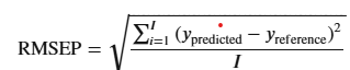
where i─no of samples; ypredicted─predicted value; and yreference─measured value.
2.2.2. Stage 2: Refining PLS-R Models to Handle a Degraded Solvent
During the second stage, important statistical parameters (23) of TIC-1 and TA-1 predictions, such as Q residuals (Q), Hotelling’s T2 (T2), and leverages were recorded to adopt the models to the degraded solvent. All the spectral samples of the MEA2 campaign were mapped in the plot of T2 versus Q which is an important tool in fault detection. Recorded prediction leverages were used to select new samples for the model updating step which is described in Section 2.2.3.2.
2.2.3. Stage 3: Applications of PLS-R Model’s Prediction Statistics for Degrading Solvent Monitoring and Management
In the third stage, three different chemometric approaches were explored to demonstrate how the PLS-R model statistical parameters can be used to update the model to stabilize predictions during the whole operation, and how the model residuals are useful for solvent management.
2.2.3.1. MSPC Demonstration
The plot of T2 versus Q of TIC-1 model is used for MSPC demonstration. Moreover, calculated Q were used to check the lack-of-fit of the models for the entire campaign period. All the results are discussed in Section 3.2.
2.2.3.2. Model Updating
TIC-1 and TA-1 models were improved for reliable long-term predictions. Here, TIC-1 and TA-1 models were converted to upgraded models (TIC-2 and TA-2) for a better predictions of in the degraded/changed solvent conditions using a calibration transfer method (26) called model updating (MUP). (27,28) In order to convert the models, a few new calibration samples were selected to describe the solvent degradation/change of the total campaign. These samples were selected using prediction leverage versus samples (time) plot, as shown in Figure 2 stage 2. These selected samples were formerly studied by visualization of spectra to identify the spectral quality of the samples, prior to incorporating them in the available models. The model updating approach comprises several iterations to arrive at properly updated prediction models (TIC-2 and TA-2). Section 3.3 discusses the results of model updating approach of TIC and TA models.
All data analysis were performed on the MATLAB platform using PLS Toolbox 8.6.2 software.
3. Results and Discussion
3.1. Preparation of Initial PLS-R Models
The use of authentic industrial data will make the PLS-R models more tolerant to the actual process variations by the assimilation of realistic dynamic process variations. In this work, initial PLS-R models (TIC-1 and TA-1) were prepared for the demonstration of the and solvent change detection and PLS-R model updating during long-term operation.
Spectral preprocessing is a significant step of PLS-R model calibration using spectroscopic data. To extract chemical species variation, specific IR bands (Figure 3) are selected to improve the ratio of signal-to-noise. Initially, all spectra were baseline-corrected using the Whittaker filter with Lambda and Rho at 1000 and 0.001, respectively. (25) The raw spectra and preprocessed spectra of the MEA2 campaign are shown in Figure 3a,b. Additionally, Figure 3b indicates the variable ranges used in the TIC (blue shade) and total alkalinity (red shade) models.

The preferred method for preparing a robust model is selection of the specific IR vibrational bands of the specific species/group to be investigated. Table 3 summarizes the main selected species, the corresponding IR bands selected for models, model variable ranges, and reference literature.
Table 3. PLS-R Model Species, Identified IR Bands, Corresponding Literature IR Bands, and Variable Ranges of the Models
| models | species | identified IR bands (cm–1) | corresponding literature IR bands (cm–1) | variable ranges of models (cm–1) |
|---|---|---|---|---|
| TIC | MEACOO– | 1562 (1) | 1568, (14,29) 1564 (30) | [1590–1467], [1407–1301] |
| 1486 (2) | 1486 (14,29) | |||
| 1320 (3) | 1322 (14) | |||
| CO32– | 1387 (4) | 1388, (14,30) 1386 (29) | ||
| HCO3– | 1362 (5) | 1360, (14,30) | ||
| total alkalinity | MEA | 1020 (6) | 1024 (14) | [1670–1590], [1113–944] |
| MEAH+ | 1638 (7) | 1634 (14) | ||
| 1067 (8) | 1069, (14) 1064, (30) 1066 (29) |
Two models (TIC-1 and TA-1) were calibrated with test set validation. The used number of samples are presented in Table 4. Figure 4a,b depict the measured versus predicted plots of TIC-1 and TA-1 models, respectively. These figures indicate that the regression line of the models (fit line: red color) sets very close to the targeted line (1:1 line: green color). Model performance indicators─model range, RMSEP, number of LVs used, and R2 predicted─are tabulated in Table 4.

Table 4. Calibration and Validation Details of the Models (TIC-1 and TA-1)
| model | number of samples | model range mol/kg | RMSEP mol/kg | LVs | R2 (pred) | |
|---|---|---|---|---|---|---|
| calibration set | validation set | |||||
| TIC-1 | 17 | 16 | 1.1–1.5 | 0.024264 | 1 | 0.977 |
| TA-1 | 13 | 13 | 4.5–5.2 | 0.039841 | 2 | 0.948 |
3.2. Follow-Up and Control of Solvent Reclaiming
Reclaiming is an important part of CO2 capture solvent management. Thermal solvent reclaiming has been practiced in the gas sweetening industry for a long time (31) and recommendations vary on the maximum allowable amount of degraded solvent/contaminants. (32) The end point of thermal reclaiming has also been connected to the reclaimer temperature. (33) In conclusion, a more detailed method for thermal reclaimer follow-up seems desirable. We assess MSPC as a potential concept for thermal reclaimer follow-up and control. MSPC is an effective concept to follow-up and control of solvent reclaiming. One of the pillars of MSPC is PLS-R models which contribute by effective extraction of the information about the solvent changes from spectroscopic data (i.e., FTIR). (23)
In this work, the T2 and Q statistics is made by mapping all T2 versus MEA2 campaign samples’ Q values of TIC-1 model predictions (Figure 5a). Furthermore, Q values of MEA2 samples were plotted versus the days of operation (Figure 5b). Figure 5a shows the process variations in the MEA2 operation. The blue shaded area holds the campaign samples which agree with solvent composition at the start of operation. The samples in the red shaded area indicate the samples deviating from the average of model population (fresh solvent condition). Increased Q values indicates increased deviation. In addition, the red dashed lines separate the 95% confidence level of Q and T2.

Figure 5a is a plot showing solvent degradation during the CO2 capture process. Figure 5b depicts that the deviation of the Q residual is drastically increasing after day 27. (Date: 23 August 2015; @around 800 h of operation). (10) This deviation of the Q residuals indicates the difference between the current solvent state and the fresh solvent. According to Morken et al., the day 27 sample consists of about 0.5 wt % of heat stable salts (HSS) based on MEA weight, 3000 mg/L of anionic IC species, and 30,000 mg/L of main amine degradation products. (10) The observations in the T2 and Q statistics (Figure 5a) agree hence with the campaign sample analytics result. Furthermore, the plot indicates that Qs of the sample recorded on the day 77 and onward decrease and finally closely resemble the calibration samples. Solvent reclaiming started on day 77 of the campaign corresponding to samples collected on 12th October 2015 at around 1852 operation hours. Furthermore, this implies that the T2 and Q statistics have the ability to detect/indicate sufficient time/extent of reclaiming of the degraded solvent.
According to Figure 5b, Q show an increasing trend in three different stages starting from mid of August 2015 until solvent reclaiming initiation on 12th October 2015. A similar trend was observed by Flø et al. by solvent viscosity measurements at two different temperatures (30 °C and 60 °C). (19) This observation demonstrates that physical solvent changes influence the solvent spectra and correlate with prediction residual spectra (Q residual). In addition, the variation of HSS concentrations displays a similar tendency. (10) Therefore, Qs are mimicking both the physical and chemical variations observed during the MEA2 campaign operation.
Although the initial PLS-R models are useful for MSPC, they must be updated during the time of operation for reliable online monitoring. In this case, the T2 and Q statistics are useful for detection of the time to update the corresponding model. The adaptation of PLS-R models for prediction of the degraded solvent system is described in the following section.
3.3. Preparation of Updated (TIC-2 and TA-2) Models
Industrial PAT applications will fail if not model adaptation is carried out during the long-term use. PLS-R model calibration transfer methods are selected consequently based on the nature of the changes in the measuring environment, i.e., chemical changes, physical changes, instrument changes, etc. An applicable model updating method for CO2 capture solvent degradation is discussed below.
Figure 6a,b illustrates the total campaign prediction models of TIC-1 and TA-1, respectively. These plots indicate that the prediction error (RMSEP) of the TIC-1 and TA-1 models are increased by 70 and 123%, respectively, as time passes. Increase of the RMSEPs suggest that these model predictions develop a higher uncertainty over time in operation. In this context, the initial calibration data set needs to be expanded to obtain stable predictions during the total campaign. In order to expand the calibration data set of the models, a sufficient number of new samples need to be integrated. This is an iterative trial-and-error method across the total run time. In selecting new samples for a model renewal, leverage or T2 values are helpful statistical parameters.

Proper sampling techniques are essential to minimize sampling uncertainties/errors. Furthermore, identification of new samples needs to be done carefully since the selected sample may have a higher tendency for being an outlier. Visual observation of raw spectra of the samples is commonly used in identifying erroneous spectra. In addition, corresponding reference values (e.g., species concentration) of the selected samples should be acquired.
TIC-1 and TA-1 models were improved by adding 9 and 8 new data, respectively. Prediction parameters of the initial models (TIC-1 and TA-1) and updated models (TIC-2 and TA-2) are tabulated in Table 5, which indicates that the RMSEPs of the updated models were reduced by about 50% compared to the initial models. In agreement with Figure 6c,d, the prediction slopes of the TIC-2 and TA-2 models are improved─0.992 and 0.957, respectively. The number of latent variables of the updated models are also limited to three components, implying that the models are more robust in the predictive nature.
Table 5. Initial Models and Updated Models’ Performance Statistics
| model parameters | TIC models | total alkalinity models | ||
|---|---|---|---|---|
| TIC-1 | TIC-2 | TA-1 | TA-2 | |
| RMSEP (mol/kg) | 0.0415 | 0.0206 | 0.0953 | 0.0514 |
| R2 (predicted) | 0.985 | 0.992 | 0.882 | 0.920 |
| LVs | 1 | 3 | 2 | 3 |
4. Conclusions
MEA speciation models from the Technology Centre Mongstad 2015 MEA 2 Test campaign were developed. On this basis, two MEA solvent monitoring models, total inorganic carbon (TIC) content and total alkalinity (TA), were prepared. In addition, the ability of the models to cope with ongoing solvent change during the test campaign was demonstrated by application of a specific model update methodology.
Finally, to the best of our knowledge, a new method for solvent monitoring and management has been discovered and demonstrated. The need for solvent reclaiming can be quantified by the combination of statistical TIC or TA prediction model residuals. This methodology also provides “start” and “end of reclaiming operation” identification.
Hence, we demonstrate using large scale test campaign data that it is possible to monitor and follow-up process performance including solvent reclaiming operation and solvent monitoring using a single spectroscopic instrument.
Further development work is in progress on the issue of reclaiming monitoring and optimization.
Author Information
- Corresponding Author
- Maths Halstensen – Department of Electrical, IT and Cybernetics, University of South-Eastern Norway, Kjølnes Ring 56, 3918 Porsgrunn, Norway; Email: Maths.Halstensen@usn.no
- Authors
- Jayangi D. Wagaarachchige – Department of Electrical, IT and Cybernetics, University of South-Eastern Norway, Kjølnes Ring 56, 3918 Porsgrunn, Norway;
 https://orcid.org/0000-0002-1544-7169
 - Zulkifli Idris – Department of Process, Energy and Environmental Technology, University of South-Eastern Norway, Kjølnes Ring 56, 3918 Porsgrunn, Norway; https://orcid.org/0000-0001-7905-9686
- Ayandeh Khatibzadeh – Department of Electrical, IT and Cybernetics, University of South-Eastern Norway, Kjølnes Ring 56, 3918 Porsgrunn, Norway
- Audun Drageset – Technology Center Mongstad (TCM-DA), 5954 Mongstad, Norway
- Klaus-J. Jens – Department of Process, Energy and Environmental Technology, University of South-Eastern Norway, Kjølnes Ring 56, 3918 Porsgrunn, Norway; https://orcid.org/0000-0002-9022-5603
- Jayangi D. Wagaarachchige – Department of Electrical, IT and Cybernetics, University of South-Eastern Norway, Kjølnes Ring 56, 3918 Porsgrunn, Norway;
- Author ContributionsThe manuscript was written through contributions of all authors. All authors have given approval to the final version of the manuscript.
- FundingThis work was funded by the Ministry of Education and Research of the Norwegian Government.
- NotesThe authors declare no competing financial interest.
Acknowledgments
The authors gratefully acknowledge the staff of TCM DA, Gassnova, Equinor, Shell, and TotalEnergies for their interest in this work and particularly for access to data from the TCM DA facility. The authors also gratefully acknowledge Gassnova, Equinor, Shell, and TotalEnergies as the owners of TCM DA for their financial support and contributions. One of the authors (K.-J.J.) would like to thank Arne Henriksen for an inspiring discussion on the use of spectral residuals.
References
This article references 33 other publications.
- Rochelle, G. T. Amine Scrubbing for CO2 Capture. Science 2009, 325, 1652– 1654, DOI: 10.1126/science.1176731 View Google Scholar
- Sodiq, A.; Hadri, N. E.; Goetheer, E. L. V.; Abu-Zahra, M. R. M. Chemical reaction kinetics measurements for single and blended amines for CO2 postcombustion capture applications. Int. J. Chem. Kinet. 2018, 50, 615– 632, DOI: 10.1002/kin.21187 View Google Scholar
- Song, J.-H.; Yoon, J.-H.; Lee, H.; Lee, K.-H. Solubility of Carbon Dioxide in Monoethanolamine + Ethylene Glycol + Water and Monoethanolamine + Poly (ethylene glycol) + Water. J. Chem. Eng. Data 1996, 41, 497– 499, DOI: 10.1021/je9502758 View Google Scholar
- DuPart, M. S.; Bacon, T. R.; Edwards, D. J. Understanding corrosion in alkanolamine gas treating plants: Part 1. Hydrocarbon Process. 1993, 72. Google Scholar
- Vevelstad, S. J.; Buvik, V.; Knuutila, H. K.; Grimstvedt, A.; da Silva, E. F. Important Aspects Regarding the Chemical Stability of Aqueous Amine Solvents for CO2 Capture. Ind. Eng. Chem. Res. 2022, 61, 15737– 15753, DOI: 10.1021/acs.iecr.2c02344 View Google Scholar
- Chahen, L.; Huard, T.; Cuccia, L.; Cuzuel, V.; Dugay, J.; Pichon, V.; Vial, J.; Gouedard, C.; Bonnard, L.; Cellier, N.; Carrette, P.-L. Comprehensive monitoring of MEA degradation in a post-combustion CO2 capture pilot plant with identification of novel degradation products in gaseous effluents. Int. J. Greenhouse Gas Control 2016, 51, 305– 316, DOI: 10.1016/j.ijggc.2016.05.020View Google Scholar
- Einbu, A.; DaSilva, E.; Haugen, G.; Grimstvedt, A.; Lauritsen, K. G.; Zahlsen, K.; Vassbotn, T. A new test rig for studies of degradation of CO2 absorption solvents at process conditions; comparison of test rig results and pilot plant data for degradation of MEA. Energy Procedia 2013, 37, 717– 726, DOI: 10.1016/j.egypro.2013.05.160View Google Scholar
- da Silva, E. F.; Lepaumier, H.; Grimstvedt, A.; Vevelstad, S. J.; Einbu, A.; Vernstad, K.; Svendsen, H. F.; Zahlsen, K. Understanding 2-Ethanolamine Degradation in Postcombustion CO2 Capture. Ind. Eng. Chem. Res. 2012, 51, 13329– 13338, DOI: 10.1021/ie300718aView Google Scholar
- Supap, T.; Saiwan, C.; Idem, R.; Tontiwachwuthikul, P. P. T. Part 2: Solvent management: solvent stability and amine degradation in CO2 capture processes. Carbon Manage. 2011, 2, 551– 566, DOI: 10.4155/cmt.11.55 View Google Scholar
- Morken, A. K.; Pedersen, S.; Kleppe, E. R.; Wisthaler, A.; Vernstad, K.; Ullestad, Ø.; Flø, N. E.; Faramarzi, L.; Hamborg, E. S. Degradation and Emission Results of Amine Plant Operations from MEA Testing at the CO2 Technology Centre Mongstad. Energy Procedia 2017, 114, 1245– 1262, DOI: 10.1016/j.egypro.2017.03.1379 View Google Scholar
- Akram, M.; Jinadasa, M. W. N.; Tait, P.; Lucquiaud, M.; Milkowski, K.; Szuhanszki, J.; Jens, K.-J.; Halstensen, M.; Pourkashanian, M. Application of Raman spectroscopy to real-time monitoring of CO2 capture at PACT pilot plant; Part 1: Plant operational data. Int. J. Greenhouse Gas Control 2020, 95, 102969, DOI: 10.1016/j.ijggc.2020.102969 View Google Scholar
- Jinadasa, M. W. N.; Jens, K.-J.; Øi, L. E.; Halstensen, M. Raman Spectroscopy as an Online Monitoring Tool for CO2 Capture Process: Demonstration Using a Laboratory Rig. Energy Procedia 2017, 114, 1179– 1194, DOI: 10.1016/j.egypro.2017.03.1282 View Google Scholar
- Grimstvedt, A.; Wiig, M.; Einbu, A.; Vevelstad, S. J. Multi-component analysis of monethanolamine solvent samples by FTIR. Int. J. Greenhouse Gas Control 2019, 83, 293– 307, DOI: 10.1016/j.ijggc.2019.02.016 View Google Scholar
- Richner, G.; Puxty, G. Assessing the Chemical Speciation during CO2 Absorption by Aqueous Amines Using in Situ FTIR. Ind. Eng. Chem. Res. 2012, 51, 14317– 14324, DOI: 10.1021/ie302056f ViewGoogle Scholar
- Kachko, A.; van der Ham, L. V.; Bardow, A.; Vlugt, T. J. H.; Goetheer, E. L. V. Comparison of Raman, NIR, and ATR FTIR spectroscopy as analytical tools for in-line monitoring of CO2 concentration in an amine gas treating process. Int. J. Greenhouse Gas Control 2016, 47, 17– 24, DOI: 10.1016/j.ijggc.2016.01.020 View Google Scholar
- Kourti, T.; MacGregor, J. F. Multivariate SPC Methods for Process and Product Monitoring. J. Qual. Technol. 1996, 28, 409– 428, DOI: 10.1080/00224065.1996.11979699 View Google Scholar
- Wise, B. M.; Gallagher, N. B. The process chemometrics approach to process monitoring and fault detection. J. Process Control 1996, 6, 329– 348, DOI: 10.1016/0959-1524(96)00009-1 View Google Scholar
- Faramarzi, L.; Thimsen, D.; Hume, S.; Maxon, A.; Watson, G.; Pedersen, S.; Gjernes, E.; Fostås, B. F.; Lombardo, G.; Cents, T.; Morken, A. K.; Shah, M. I.; de Cazenove, T.; Hamborg, E. S. Results from MEA Testing at the CO2 Technology Centre Mongstad: Verification of Baseline Results in 2015. Energy Procedia 2017, 114, 1128– 1145, DOI: 10.1016/j.egypro.2017.03.1271 View Google Scholar
- Flø, N. E.; Faramarzi, L.; de Cazenove, T.; Hvidsten, O. A.; Morken, A. K.; Hamborg, E. S.; Vernstad, K.; Watson, G.; Pedersen, S.; Cents, T.; Fostås, B. F.; Shah, M. I.; Lombardo, G.; Gjernes, E. Results from MEA Degradation and Reclaiming Processes at the CO2 Technology Centre Mongstad. Energy Procedia 2017, 114, 1307– 1324, DOI: 10.1016/j.egypro.2017.03.1899 View Google Scholar
- Gjernes, E.; Pedersen, S.; Cents, T.; Watson, G.; Fostås, B. F.; Shah, M. I.; Lombardo, G.; Desvignes, C.; Flø, N. E.; Morken, A. K.; de Cazenove, T.; Faramarzi, L.; Hamborg, E. S. Results from 30 wt% MEA Performance Testing at the CO2 Technology Centre Mongstad. Energy Procedia 2017, 114, 1146– 1157, DOI: 10.1016/j.egypro.2017.03.1276 View Google Scholar
- 21Hjelmaas, S.; Storheim, E.; Flø, N. E.; Thorjussen, E. S.; Morken, A. K.; Faramarzi, L.; de Cazenove, T.; Hamborg, E. S. Results from MEA Amine Plant Corrosion Processes at the CO2 Technology Centre Mongstad. Energy Procedia 2017, 114, 1166– 1178, DOI: 10.1016/j.egypro.2017.03.1280 View Google Scholar
- Bui, M.; Flø, N. E.; de Cazenove, T.; Mac Dowell, N. Demonstrating flexible operation of the Technology Centre Mongstad (TCM) CO2 capture plant. Int. J. Greenhouse Gas Control 2020, 93, 102879, DOI: 10.1016/j.ijggc.2019.102879 View Google Scholar
- Esbensen, K. H.; Swarbrick, B., Multivariate Data Analysis : An Introduction to Multivariate Analysis, Process Analytical Technology and Quality by Design. 6th ed.; CAMO software AS: 2018.Google Scholar
- Wold, H. Soft Modelling by Latent Variables: The Non-Linear Iterative Partial Least Squares (NIPALS) Approach. J. Appl. Probab. 1975, 12, 117– 142, DOI: 10.1017/s0021900200047604 View Google Scholar
- Eilers, P. H. C. A Perfect Smoother. Anal. Chem. 2003, 75, 3631– 3636, DOI: 10.1021/ac034173t View Google Scholar
- Workman, J. J. The Essential Aspects of Multivariate Calibration Transfer. 40 Years of Chemometrics – From Bruce Kowalski to the Future; American Chemical Society, 2015; Vol. 1199, pp 257– 282. View Google Scholar
- Wise, B. M.; Roginski, R. T. A Calibration Model Maintenance Roadmap. IFAC-PapersOnLine 2015, 48, 260– 265, DOI: 10.1016/j.ifacol.2015.08.191 View Google Scholar
- Tan, H.; Sum, S. T.; Brown, S. D. Improvement of a Standard-Free Method for Near-Infrared Calibration Transfer. Appl. Spectrosc. 2002, 56, 1098– 1106, DOI: 10.1366/000370202321275015 View Google Scholar
- Sun, C.; Dutta, P. K. Infrared Spectroscopic Study of Reaction of Carbon Dioxide with Aqueous Monoethanolamine Solutions. Ind. Eng. Chem. Res. 2016, 55, 6276– 6283, DOI: 10.1021/acs.iecr.6b00017 View Google Scholar
- du Preez, L. J.; Motang, N.; Callanan, L. H.; Burger, A. J. Determining the Liquid Phase Equilibrium Speciation of the CO2–MEA–H2O System Using a Simplified in Situ Fourier Transform Infrared Method. Ind. Eng. Chem. Res. 2019, 58, 469– 478, DOI: 10.1021/acs.iecr.8b04437 View Google Scholar
- Kohl, A. L.; Nielsen, R. B. Gas Purification; Gulf Professional Publishing: Houston, 1997. View Google Scholar
- Dumée, L.; Scholes, C.; Stevens, G.; Kentish, S. Purification of aqueous amine solvents used in post combustion CO2 capture: A review. Int. J. Greenhouse Gas Control 2012, 10, 443– 455, DOI: 10.1016/j.ijggc.2012.07.005 View Google Scholar
- ElMoudir, W.; Supap, T.; Saiwan, C.; Idem, R.; Tontiwachwuthikul, P. Part 6: Solvent recycling and reclaiming issues. Carbon Manage. 2012, 3, 485– 509, DOI: 10.4155/cmt.12.55
Cited By
This article is cited by 2 publications.
- Jayangi D. Wagaarachchige, Zulkifli Idris, Ayandeh Khatibzadeh, Audun Drageset, Klaus-Joachim Jens, Maths Halstensen. Demonstration of CO2 Capture Process Monitoring and Solvent Degradation Detection by Chemometrics at the Technology Centre Mongstad CO2 Capture Plant: Part II. Industrial & Engineering Chemistry Research 2024, 63 (24) , 10704-10712. https://doi.org/10.1021/acs.iecr.4c00019View
- Arash Sadeghi, Mohammad Reza Rahimpour. Carbon capture by solvents modified with nanoparticle. 2024, 105-124. https://doi.org/10.1016/B978-0-443-19233-3.00016-XView