
3. Development of CO2 capture process cost baseline for 555 MWe NGCC power plant using standard MEA solution (2022)
Koteswara Rao Puttaa*, Daniel Saldanab, Matthew Campbella, Muhammad Ismail Shaha
aTechnology Centre Mongstad, 5954 Mongstad, Norway
bAspen Technology, Inc, 01730 Bedford, Massachusetts, USA
Abstract
Carbon capture, utilization and storage (CCUS) is essential to achieve Net-zero emissions targets. The IEA sustainable development scenarios also emphasize the importance of CCUS. Post-combustion CO2 capture using amine solvents is the most mature technology among several options available and amine-based CO2 capture projects have been demonstrated at industrial scale. Several new vendors and technology developers are working on multiple innovative and advanced CO2 capture concepts. Industrial clients, project developers targeting the CO2 capture projects in their facilities require reliable and updated costing information using non-proprietary solvents to develop investment strategies, portfolios and evaluate the commercial project bids for CO2 capture.
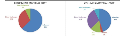
The CO2 project cost estimation depends on several factors like solvent used, amount of flue gas treated, accuracy of the simulation tool/model used for designing the CO2 capture plant, quality and size of experimental pilot data used for model validation, accurate representation of the capture facility while keeping the columns hydraulics suitable for practical operation, consideration of space requirements for column internals, design of plate heat exchangers and other packaged items like filter package and reclaiming units. Domain knowledge and practical operational experience are also crucial to perform the study. Selection of appropriate material of construction also plays a key role in accuracy of cost estimation. Technology Centre Mongstad’s 10 years of operational knowledge and experience together with AspenTech’s expert team worked together to perform a reliable and accurate costing exercise by considering all essential elements of CO2 capture process and project. The key finding from the current costing baseline study are columns material costs found to account for 63% of total CO2 capture process equipment material costs and absorber alone accounts for 45% of these total equipment material costs. The total capital expenditure for capturing 90% CO2 from 555 MWe Natural Gas Combined Cycle (NGCC) power plant using aq. 30 wt% MEA solvent is estimated to be around 326.6 Million USD. Annual total operating costs are estimated to be 47 Million USD. Assuming 25 years of plant life, the cost of CO2 capture is calculated to be 47 USD/ton.
1. Introduction
The CO2 Technology Centre Mongstad (TCM) is located next to the Equinor Mongstad refinery in Norway. TCM DA is a joint venture owned by Gassnova representing the Norwegian state, Equinor, Shell, and TotalEnergies. TCM is the largest post-combustion CO2 capture (PCC) test centers in the world. This facility has been in the operation from 2012 and is often called the “amine plant”.
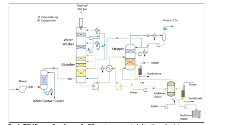
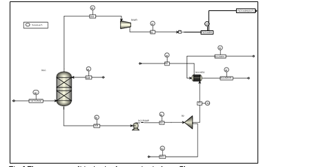
TCM amine plant was built to run on two different types of flue gases, namely, natural gas-fired combined heat and power (CHP) plant i.e., CHP flue gas is from a natural gas fired CCGT plant or the Equinor Mongstad refinery residue fluid catalytic cracker (RFCC). Over the last 10 years, several commercial vendor proprietary solvents as well as non-proprietary solvents have been tested at TCM amine facility. TCM amine plant is well equipped with around 4,000 online sensors to gather critical information in addition to more than 100 offline manual sampling points. TCM has more than 20,000 hours non-proprietary operational data using aqueous monoethanolamine and CESAR 1 (AMP/PZ mixture) [1–7]. Fig. 1 shows the process flow diagram for CO2 capture process at TCM.
A comprehensive baseline for performance and cost estimation of CO2 capture processes is crucial to assess, identify and support widespread deployment of CO2 capture projects. Successful CCUS (Carbon Capture Utilization and Storage) projects will be essential for achieving world Net-Zero emissions targets by 2040-2050. To have a fair assessment of new technology developments and avoid using commercial technology as baseline, TCM has developed a cost baseline using a non-proprietary solvent, i.e., aqueous 30 wt% Monoethanolamine (aq. MEA) solution. The assessment of performance and cost were determined independently and does not represent the views of any technology vendor. The baseline input conditions for this model and costing exercise were based on National Energy Technology Laboratory (NETL) baseline study case 14 [8] with CO2 capture.
The present work discusses about the systematic methodology or steps followed to develop a technoeconomic analysis (TEA) for CO2 capture technology using AspenTech products like Aspen Plus, Aspen EDR, Aspen Capital Cost Estimator (ACCE). A proper costing baseline development must contain five critical steps, given below:
Step 1: Develop and validate an accurate rate-based process model with operational data from pilot plant Step 2: Run steady state simulation with aqueous 30 wt% MEA solvent targeting 90% CO2 capture from the industrial plant of interest and capacity
Step 3: Perform detailed sizing of major process equipment such as columns (direct contact cooler, absorber, regenerator, water-wash sections) and heat exchangers, pumps, blower/compressors …etc.
Step 4: Perform estimation of costs using vendor quotes and/or relevant costing software tools by considering all relevant elements
Step 5: Economic/financial analysis and presentation of results and sensitivity study
These steps are described in detail in the following sections 2 and 3.
2. Methodology
As mentioned above, a proper technoeconomic analysis for CO2 capture technology using alkanolamines requires five essential steps explained below.
In the present work, CO2 capture using aqueous MEA solution has been considered and AspenTech software tools are used to perform different steps involved in the TEA. In this section, Steps 1- 4 will be described in detail and step 5 will be presented in section 3.
2.2 Step 1 – Development and validation of process model
In order to develop the process model, it is important to understand the chemicals used, chemistry involved and phenomena occurring in the process. Thermodynamics plays key role in CO2 absorption process design and simulation as the absorption with chemical solvents requires thermodynamic data, especially phase equilibria: vapor-liquid equilibrium (VLE) and speciation in the solution. Aqueous amine systems used for CO2 capture are non-ideal systems which can be thermodynamically modelled utilizing activity coefficients models for the liquid phase such as Electrolyte NRTL (e-NRTL), Extended-UNIQUAC or similar. Gas phase is modelled by utilizing equation of state such as Redlich-Kwong (RK) or Soave-Redlich-Kwong (SRK). Aspen Plus V11 software is used to develop the model and validate.
In the current study, MEA is the main chemical used as solvent to capture the CO2 from flue gas. In the present study, e-NRTL RK method has been chosen for thermodynamic modelling. The chemistry/ chemical equilibrium involved in the MEA-CO2-H2O system are given by the reactions (1)-(5) below [9,10].
Ionization of water:
2H2O ↔ OH− + H3O+ (1)
Dissociation of carbon dioxide:
2H2O + CO2 ↔ H3O+ + HCO3− (2)
Dissociation of bicarbonate:
H2O + HCO3− ↔ H3O+ + CO32− (3)
Dissociation of protonated amine:
MEAH+ + H2O ↔ H3O+ + MEA (4)
Carbamate reversion to bicarbonate:
𝑀𝐸𝐴𝐶𝑂𝑂− + 𝐻2𝑂 ↔ 𝑀𝐸𝐴 + 𝐻𝐶𝑂3− (5)
In the literature, simulation or design of columns is performed by either using equilibrium-based approach or rate- based modelling approach. For CO2 capture applications with amine solvents, rate-based modelling approach gives a more realistic and predictive model compared to equilibrium-based approach. Rate-based modelling approach has been used for all columns in the CO2 capture.
In addition to the reactions (1)-(5) considered in equilibrium thermodynamic model above, kinetic reactions are also important to accurately design and simulate the process, especially absorber column. Two reactions have been considered to be kinetically controlling, given below [9,11,10]:
𝐶𝑂2 + 𝑂𝐻− ↔ 𝐻𝐶𝑂3− (6)
𝐶𝑂2 + 𝑀𝐸𝐴 + 𝐻2𝑂 ↔ 𝑀𝐸𝐴𝐶𝑂𝑂− + 𝐻3𝑂+ (7)
Power law expressions are used for the rate-controlled reactions (reactions (6)- (7)) on activities basis. The power law expression (8) is used for reaction rate:
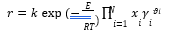
Where 𝑟 represents reaction rate; 𝑘 is pre-exponential factor; 𝐸 is activation energy; 𝑅 is Universal gas constant; 𝑥𝑖 is mole fraction of component i; 𝛾𝑖 is activity coefficient of component i; 𝜗𝑖 is the stoichiometric coefficient of component i in the reaction equation and T is temperature. Kinetic reaction parameters are regressed using literature kinetic data.
After the development of the e-NRTL RK thermodynamic model for MEA-CO2-H2O system and kinetic parameters refinement to match literature data, this model is validated with TCM testing pilot scale data. This validation has been performed by implementing TCM amine plant in Aspen Plus and collecting the steady state operational data over wide range of conditions. The operating conditions window used for the model validation is given in Table 1. The criteria for selection of steady state conditions employed in model validation are as follows:
- Overall plant mass balance is 100 +/- 2%
- CO2 mass balance 98 +/- 2%
- Stable operation at least 2 – 6 hours (steady state operation)
- Availability of liquid lab analysis results for CO2 and amine concentrations
Table 1 TCM Aspen Plus model validation conditions range for CO2 capture using aq. MEA solution
| Operating parameter | units | Range |
| Flue gas flowrate | Sm3/hr | 34,000 – 68,000 |
| Flue gas CO2 concentration | vol % | 3.6 – 14 |
| Flue gas temperature | oC | 28 – 45 |
| MEA concentration | wt % | 28 – 40 |
| Lean amine loading | mol/mol | 0.1 – 0.3 |
| Lean amine temperature | oC | 35 – 50 |
| CO2 capture rate | % | 70 – 99 |
| Absorber packing height | m | 12,18, 24 |
| Water wash sections | # Sections | 1, 2 |
| Stripper in operation | – | CHP, RFCC† |
† The difference between CHP and RFCC strippers is in the diameter. CHP stripper ID=1.25 m and RFCC stripper ID=2.2 m. Both strippers are The model validation results are shown in Fig. 2. As it can be seen from the Fig. 2, the model predicts the pilot scale data with good accuracy both for CO2 capture as well as specific reboiler duty (SRD). The outliers or higher deviation in the SRD corresponds to cases where maldistribution and foaming were occurring in the stripper during operation.
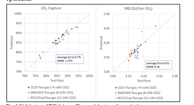
After extensive validation with TCM scale pilot data and proven model predictability over wide range of operation window, the TCM Aspen plus model is used for simulating and designing real industrial scale plants.
2.2 Step 2 – Simulation of CO2 capture from NGCC power plant
The present study is to capture CO2 from 555 MWe Natural Gas Combined Cycle (NGCC) power plant. Aqueous 30 wt% MEA solution is used as solvent for capturing CO2. Steady state simulation with aqueous 30 wt% MEA solvent targeting 90% CO2 capture from 555 MWe‡ Natural Gas Combined Cycle (NGCC) power plant. This was based on the case 14 from NETL baseline reference [8] performed with MEA solvent. The flue gas conditions are given in Table 2.
The validated model described in section 2.1 using Aspen plus is used to simulate the design case. The process description for CO2 capture is given in the following paragraphs.
Table 2 555 MWe NGCC plant flue gas conditions for CO2 capture
| Name | Value | Units |
| Flow rate | 113,831 (3,230,636) | kgmol/hr (kg/hr) |
| T | 143 | °C |
| P | 0.1 | MPa, abs |
| Annual operation | 8000 | hours |
| Capture rate | 90 | % |
| Annual CO2 capture | 1,475, 200 | ton/year |
| Composition | Mole fraction | |
| Ar | 0.0089 | |
| CO2 | 0.0404 | |
| H2O | 0.0867 | |
| N2 | 0.7432 | |
| O2 | 0.1209 | |
| NOX | 155 | ton/year |
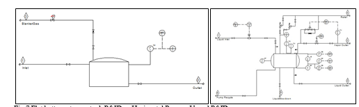
Flue gas from the NGCC power plant is introduced in direct contact cooler (DCC) to cool it to the required absorber inlet temperature. In the DCC cold water is feed at the top and hot flue gas (143°C) is introduced at the bottom of the DCC column. The flue gas moves counter-current to the cold water over a packed section and gets cooled to the desired temperature and leaves to the absorber via a flue gas blower. The flue gas blower supplies enough pressure to the flue gas to overcome the pressure drop in the absorber. In the DCC, when the incoming flue gas is cooled by contacting with the cold water, water vapor in the flue gas gets condensed. The excess water condensed from flue gas will be bled and the remaining water will be cooled in the DCC water cooler (DCCHEX) and sent back to the DCC top. The flue gas cooling process implementation in Aspen Plus is shown in Fig. 3.
The pre-conditioned flue gas from DCC is fed to the absorber bottom where it meets counter-currently the lean amine fed at the top of absorption section. CO2 is captured by amine via an exothermic reaction forming a carbamate as MEA is primary amine. The lean amine becomes richer and richer as it flows down the absorber column and leaves the absorber bottom via rich amine pump to the stripper via rich/lean cross plate heat exchanger. The flue gas becomes depleted in CO2 on its way upward in the absorber column, due to exothermic reactions in the absorber, the flue gas and amine solvent temperature increases. The NGCC flue gas leaving the absorption section is normally saturated with water and containing volatile components like solvent amine and other amine degradation products. To reduce loss of amine and reduce emission of volatile components such that the plant can be operated within regulated emission permit, the flue gas from the absorption section needs to be cooled and conditioned water washes sections above of the absorber section before sending it to the atmosphere via flue gas stack. In the water wash sections, the flue gas is cooled by counter current flow of cold water, which partially condenses water and some of the volatile components. The condensed stream is fed back either to the bottom of the absorber or can be fed with lean amine feed to the absorber to keep the plant in water balance and reduce the amine loss.
In the stripper the CO2-rich amine solution flows downwards during which CO2 is stripped off from the rich solution by supplying heat in a reboiler with low pressure steam. The CO2-rich gas stream containing CO2, steam, and solvent vapor from the top of the stripper is partially condensed in the overhead condenser and separated from the gas stream in the gas-liquid separator. The condensed liquid is sent to the stripper using reflux pump. The top section of the stripper is a wash/rectification section designed to limit the amount of solvent vapor entering the stripper overhead system.
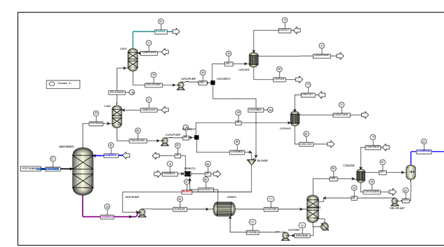
The stripped solvent from the bottom of the stripper, i.e., CO2-lean solution from the bottom of the stripper is cooled-down in the lean/rich cross heat exchanger after heat exchange against the rich solvent; further cooled in the lean amine cooler to achieve the desired temperature for the optimal operation of the absorber. However, solid particles from the feed flue gas could get into the solvent and cause foaming during operation. A split stream of about 5-10% of the circulating solvent is passed through a filtration unit consisting of a mechanical pre-filter, activated carbon bed and post-filter, to remove solid particles and substances that could increase foaming in the solvent. Aspen plus V12 implementation of CO2 capture process is shown in Fig. 4.
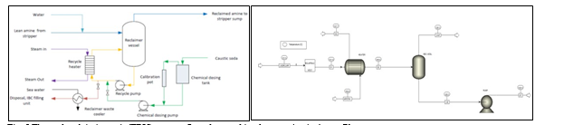
Amine based solvents will degrade over time, the rate of degradation is depending on the solvent molecular stability, flue gas contaminants more specifically NO2, SO2 and O2, operating conditions and plant design (hot inventory). The level and composition of corrosion and solvent degradation products also affect the degradation rate. Capture, HSE and energy performance of the solvent will deteriorate over time unless the solvent is kept in good hygiene to reduce the degradation. One way of keeping the solvent is reclaiming, where a slip stream (normally a slip from hot lean amine stream downstream lean amine pump) is reclaimed in a thermal reclaimer unit (TRU). Reclaiming is performed at higher temperatures than stripper (130-150°C for MEA). Caustic soda (NaOH) is added to the recycle stream to neutralize the acids and liberate MEA. The amount of caustic to inject can be calculated based on the amounts of organic acids (formic, glycolic, oxalic, and acetic), nitrate, nitrite, and sulfate in the solvent. Due to high temperature, water and major portion of the non-degraded amine are evaporated and fed back to the stripper via top of the TRU. The bottom of the TRU contains heavy molecules, some solvent amine and most of the degradation products. These bottoms products are more viscous than solvent amine and are pumped out and disposed as hazardous waste depending on the composition. The reclaiming section schematic and implementation in Aspen Plus is shown in Fig. 5.
2.3 Step 3 – Equipment sizing
After simulation the CO2 capture unit, the next step is to perform sizing of all essential equipment. This sizing information will be utilized in the next cost estimation step. This section provides some key information and tools
used to perform sizing of different equipment.
- Columns: As Aspen Plus rate-based model is used to perform the simulation in Step 2 above, diameter and packing height is calculated from the Aspen Plus for the selected packing by maintaining good hydrodynamics and meeting the design requirements. In the costing, as the tangent-to-tangent information needs to be provided to get accurate/reliable price for the columns, the spacing required for the internals (e.g., demisters, liquid collectors and distributors, packing supports, sump … etc.) in the columns was calculated based on TCM amine plant columns.
- Plate heat exchangers: The process information from the Aspen Plus simulation is transferred to the Aspen Exchanger Design and Rating (EDR) V12 software and exchanger sizing was performed using the EDR tool to meet the required heat transfer duties and achieve corresponding temperatures for the process/utility streams. The plate types in the plate heat exchangers are selected based on the TCM internal datasheets from the amine plant.
- Reboiler: Kettle type reboilers were designed in the EDR software using the solvent and steam information from the Aspen Plus simulation.
- Separators/vessels: Gas -liquid Separators, reclaimer vessel sizing was performed using Aspen Plus sizing feature.
- Storage tanks: Storage tanks sizes for solvent storage, Caustic storage, reclaimer waste storage was estimated from volume of liquids/solvents from process simulation as well as process operating experience from TCM.
- Cooling towers: Cooling duties and cooling water flowrate were taken from the Aspen Plus simulation performed in step 2. Using this information and cooling towers standards, cooling tower units sizing was considered by discussing with experts working in the industry.
- Filtration unit: Activated carbon filter package sizing was performed assuming that a slip stream of lean amine solvent, i.e., 10% of lean solvent will be sent to filter package.
In addition to the AspenTech softwares, TCM internal tool for reclaimer and TCM internal database have been used in the present study.
2.4 Step 4 – Cost Estimation
This section provides information and methodology followed to estimate the costing using Aspen Capital Cost Estimator (ACCE) V12 software. Step 4 has been performed together with experts from AspenTech. The cost estimations in this work represent the costs that are relative to new plants without considering specific project requirements for design, standards or site integration
AspenTech’s Economic Evaluation solution is based on a core design, estimating, scheduling, and expert systems technology. It automatically develops preliminary design-based economic results – early from minimal scope, and refined designs and economics later in the project. This unique technology provides:
- Key answers quickly
- Dramatic reductions in evaluation time and resources
- The best, most economical process and plant design for funding/bidding decisions and project evaluation.
Aspen economic evaluation systems (including Aspen Capital Cost Estimator and Aspen Process Economic Analyzer) are in daily use. Aspen Capital Cost Estimator uses the equipment models contained in the Evaluation Engine – a knowledge base of design, cost, and scheduling data, methods, and models – to generate preliminary equipment designs and simulate vendor-costing procedures to develop detailed Engineering-Procurement- Construction (EPC) estimates. Volumetric models generate a costed, quantity takeoff for the bulk materials without using factors or user input. The volumetric models also produce the quantities of pipe, valves, concrete, steel, and instruments identified by the associated equipment or area. Components of each line of pipe and instrument loop are quantified and costed, enabling the user to view and adjust construction tasks. The Aspen Capital Cost Estimator Work Item Models produce the required man-hours by craft and task needed to install Aspen Capital Cost Estimator- generated bulks, as well as the equipment Aspen Capital Cost Estimator designed, by simulating detailed design construction tasks. Finally, the Engineering Models in Aspen Capital Cost Estimator produce man-hours by discipline and engineering work product.
Cost indices in the economic evaluation suite and Aspen Capital Cost Estimator include engineering disciplines, wage rates, material costs, shop and field labor rates, construction equipment rental rates, etc. These indices do not derive from public sources, and they may not accurately reflect how they affect a specific project. To evaluate this, the user should run benchmark projects and develop own adjustments.
2.4.1 Aspen Capital Cost Estimator Project General Workflow
- Create project scenario and define properties like country base, units of measure, and currency.
- Define design basis (general mechanical design rules), wage rates and productivities, code of account definition and allocation, material and man-hour indexing, equipment rental, and project execution schedule settings.
- Define the Power Distribution system (if desired).
- Define the Process Control system (if desired) and link to areas and substations.
- Add contractors and redefine responsibilities (if desired) and link to areas and substations.
- Run an item evaluation to produce direct costs for an individual component or run a project evaluation to produce design and cost results needed to prepare project reports.
- View and/or print reports.
2.4.2 Generating the economic evaluation for this project
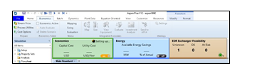
The economic evaluation project with the equipment list can be generated in simulation either within the simulation itself or by importing the simulation file into ASPEN CAPITAL COST ESTIMATOR. The economic evaluation can be started from within the simulation, by setting the economics active in the economic evaluation tab, as shown in Fig. 6.
The simulation will generate a preliminary estimate based on default values; however, these values should be reviewed by the user. The first thing to review will be the mapping process.
Simulations and estimates differ in the sense that a theoretical unit operation is not the same as pieces of equipment set on a plant. For example, a column unit operation may converge for heat and mass balance, but when estimating it, an actual distillation process needs the column vessel, the reboilers, the condensers and accumulators as well as the pumps to circulate the condensate. Furthermore, mapping is important because while a heat exchanger may be represented by a simple unit operation, for estimation it will be very important to define if the type is an air cooler, shell and tube exchanger or others. Lastly, the mapping exercise will also have an impact on the bulks cost calculated by the economic evaluation engine for example a separator in a simulation may represent a process vessel or a storage tank and these will have greatly different impact in the piping and instrumentation associated to each of them as shown in Fig.7.
As the Fig.7 illustrates below, a horizontal process vessel needs more piping and instrumentation items than a general storage tank would. This has an impact in the final estimated project cost.
Once the mapping exercise is done the, the economic evaluation technology integrated in the simulation will perform a sizing of the equipment list generated in the previous list. This sizing considers the mass and energy balances calculated in the simulation and sizes the equipment following standards defined in the design bases under “cost options”. Design Basis defines the general mechanical design rules for the entire project. AspenTech’s Economic Evaluation uses built in, industry-standard design procedures for the preparation of mechanical designs. The standards used include ASME (American Standards), BS5500 (British Standards), JIS (Japanese Standards), DIN (German Standards), or EN 13445 (European Standards).
Finally given the equipment list and design generated in the economic evaluation, a preliminary cost analysis will be generated for the equipment listed in the simulation which includes the material cost as well as the installed cost of the equipment list, it will also include a preliminary operational cost given the utilities defined in the simulation (ACCE has default utilities defined in case a user does not define them manually) and generates an “IZP” file that is readable by Aspen Capital Cost Estimator, AspenTech’s detailed estimating tool.
It is important to mention that an estimate generated from the simulation and the cost results displayed in the simulation are just a preliminary cost. For an asset’s total install cost (TIC) to be completely estimated, it still needs definitions of structures such as Pipe Racks, the Piping that will interconnect multiple areas, Control Centers, Power Distributions, any and all skids for the dosage packages etc. User input is required for labor wage rates, productivities, escalation indexes, utilities cost definitions, licensor and other indirect costs, contingency costs, etc. For this, previously generated IZP file is imported into Aspen Capital Cost Estimator and add more details to the existing estimate to create a higher quality estimate that can be backed up with better data.
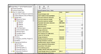
Open the IZP file in Aspen Capital Cost Estimator and review the Project Basis. So far, default values have been used, however have more control within the Aspen Capital Cost Estimator User Interface to adjust and modify the cost and design basis to meet the needs.
In the Equipment Specs form under Design Basis, design information specific to the project needs to be entered, such as:
- Design allowances
- Rental equipment option for lifting
- Shop fabrication specifications
- Design cut off temperature
Notice default values are light blue colored while user entered values will be black as shown in Fig. 8.
Continuing under Project basis view, user will find General Piping Specs form. Enter here information such as Pipe fabrication preferences, tracing tube material, X-ray analysis percentage, insulation jacket material, etc.
As moving on to the next form Civil/Steel Specs will be displayed. This form will let the user enter information about plant site such as soil type, loading density, wind velocity, pile types and sizes. All this data is used to calculate the amount of civil work needed to setup the equipment, for example how much foundation the columns need as well as structural steel, all key parts of the direct cost estimated.
Continuing, next to the Instrumentation Specs Form. This form allows the user to enter information about the instrumentation configuration needed in the project, such as P&ID design, Instrumentation type and system, Junction Box distances and cable size option. Entering this information will affect the quantity of material needed for instrumentation, the type of material used and will directly affect the Instrumentation code of account direct cost. The most important modification done for this project will be the type of instrumentation, as the default Pipe and Instrumentation design (P&IDs) is changed from Standard Instrumentation to Fully Instrumented (FULL). One important point to consider here using the domain knowledge, even the fully instrumented option still doesn’t have all the required instrumentation for few equipment, such as absorber column which contains both absorption and water wash sections in the same column. User needs to add additional instrumentation required manually. This option is available in ACCE.
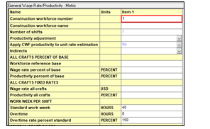
Wage Rates form is available under the Construction Workforce folder. This form shown in Fig. 9 allows to enter data for wage rates, productivities, shifts per workday, overtime wage rates. This information is used to calculate the total labor hours needed to install all equipment and bulks, reflected in the direct costs.
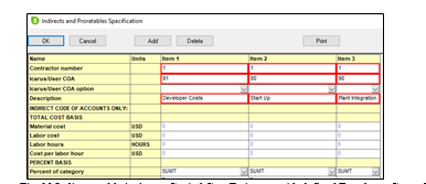
To add Indirect cost such as Developer Cost, Plant Integration and Start Up as a percentage of the EPC cost, user can add them to the “Indirect Prorate-able” table, in this table users are able to define costs as percentage basis of the EPC cost and can also organize said costs as direct costs by defining its “code of account” a code that allows for reporting purposes where should the cost be displayed. An example of how this table looks can be seen in Fig. 10.
Moving into Project basis, there are other aspects of an EPC estimate that have been not considered so far. The Aspen Plus simulation link with Economic Evaluation gave us the major pieces of equipment present in the project, however items such as pipe racks, interconnecting piping with the outside battery limits, motor control centers, and even services such as dosage packages and cooling towers are not present in a normal simulation but are important to be considered when evaluating the capital cost of a project. Items can be added manually from the Aspen Capital Cost Estimator library of components as shown in Fig. 11.
For items like the dosage packages, user can add them as vessels and pumps that are mounted on skids. ACCE allows us to add these skids and reuse them in future projects as new library items.
Once user has completed the scope of the direct costs entered in Project View and the Indirect Costs entered in Project Basis, user can evaluate the estimates to generate reports to give the CAPEX of the project.
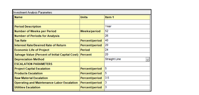
To analyze the OPEX of the project is important to correctly define the Investment Parameters form for the asset. The Economic Evaluation soluition provides a standard form with data, but defining correctly the Economic Life of the Project, the number of years and how many weeks per year, will be important for this analysis. User should also define how many hours will the asset will be operating per year as shown in Fig. 12.
It is important to set-up operating unit costs, that allows to define operator and supervision costs that will be needed year over year to operate the asset/plant. Raw material cost is also necessary for this analysis, in this case, defining the cos of the MEA will be key. Lastly defining the utilities costs for steam, cooling water, electricity and intrumentation air will allow the software incorporate these costs into the Investment Analysis and provide a breakdown of the costs year over year of the asset.
3. Results and Discussion
After finishing the step 4, the user needs to evaluate the project in ACCE to get costing report for the project. The user has the possibility to select interactive excel based report. ACCE will generate extensive report with 99 different types of summaries related to the project. In this section (step 5), the main focus will be on the results generated/estimated from the economic analysis to get insights like capital and operating costs and cost of CO2 capture per ton. The cost basis used for economic analysis in ACCE V12 is 2019 Q1. This is considered as base year for TCM costing estimations.
The Capital cost summary with various details, estimated by ACCE is shown in Fig. 13 below. The total capital cost (referred to as Project Total Costs in ACCE and Fig. 13) for capturing 90% CO2 from 555 MWe Natural Gas Combined Cycle (NGCC) power plant using aq. 30 wt% MEA solvent, estimated by ACCE is around 326.6 MUSD. The equipment cost (~105 MUSD) corresponds to 32% of Project Total Costs.
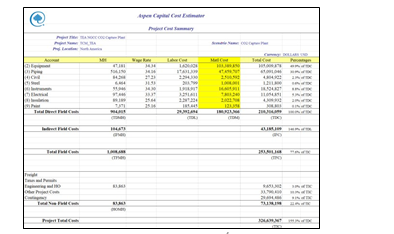
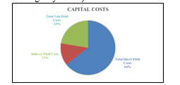
The direct and indirect field costs summary is shown in Fig. 14. Direct field costs contribute to 64% of total capital costs. Direct field costs include equipment, piping and instrumentation, civil and steel structures, insulation, and paint required. Indirect field costs include scaffolding, consumables like small tools and consumable materials, construction rental equipment costs, startup and commission, field supervision …etc. Non-field costs include engineering costs (basic, detailed engineering and materials procurement, contract fees, general, and administrative overheads, and contingency …etc.)
§ According to the current market data, the cost for plate heat exchangers is overestimated in ACCE V12. This can be modified by recalibrating the plate heat exchangers costs in ACCE using vendor quotes. This calibration was performed by using costing data from CO2 capture projects, calculating the over-estimation factor and indexing the data accordingly, matching market data.
The materials cost summary of CO2 capture plant is shown in Fig. 15. Columns material costs account for 63% of total equipment material costs and absorber accounts for 45% of total equipment material costs.
In order to understand and verify the accuracy of the cost estimates from the present work, a comparison has been made with NETL baseline study cost estimates [8]. In the NETL baseline study, flue gas pre-conditioning is not considered. Therefore, a comparison is made after excluding the flue gas pre-conditioning section (all associated equipment) which represent a reduction of 18% of the total equipment costs. The CAPEX for equipment (total field costs) estimated by ACCE is around 172.8 MUSD and prorating the NETL baseline costs using the chemical engineering plant cost index (CEPCI) estimated to be around 162.1 MUSD. This translates into 6.5% increase in costs, which is an acceptable deviation, as shown in Table 3.
Table 3 TCM Aspen and NETL baseline cost estimates comparison
| Name | TCM | NETL |
| Cost base | 2019 Q1 | 2007 June |
| Capital costs excluding flue-gas pre-conditioning (direct), MUSD | 172.8 | 140.0 |
| Prorated costs to TCM base year, MUSD | – | 162.1 |
| Difference (%) | – | 6.5 |
Operating costs for the CO2 capture plant will include costs for manpower, utilities (cooling water, steam, process water), power and solvent makeup, other chemicals and waste handling costs. It is assumed that on annual basis, cooling water make-up will be 10% to compensate for bleed. Solvent costs will require an estimate of solvent lost due to degradation, evaporation losses as well as solvent lost in the waste during reclaiming. TCM internal tool for reclaiming has been used to estimate the annual total solvent makeup required. Solvent and reclaimer waste handling costs are taken from TCM internal quotes.
The total annual operating costs are estimated to be 47 MUSD. With MEA cost of 2000 USD/ton, the solvent makeup costs account for 15% of the total operating costs and these costs share increases to 20% with 3000 USD/ton MEA price. Solvent degradation is very crucial when it comes to optimizing the CO2 capture projects operating costs.
Cost of CO2 capture per ton:
Cost of CO2 capture per ton is calculated using the following equation (9) [12].
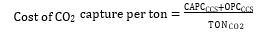
Where CAPCCCS represents annualized capital investment costs and OPCCCS represents annual operational costs of CO2 capture plant and TONCO2 represents tons of CO2 removed in a year.
With 25 years of plant life and 5% discount rate, the cost of CO2 capture per ton is calculated to be 47 USD and the cost increases to 50 USD with 3000 USD/ton MEA solvent price, i.e., 6.4 % increase.
4. Conclusions
An extensive study has been conducted by Technology Centre Mongstad together with AspenTech to develop CO2 capture process cost baseline for 555 MWe NGCC power plant using non-proprietary 30 wt% MEA solution as solvent to guide project developers as well as new technology developers to assess the project feasibility as well as merits of new technologies.
This study explains in detail all the essential steps involved in developing a cost baseline starting from the model development, validation with pilot scale operational data, simulation of process at the desired scale, detailed equipment design, project costs estimation and finally analysis of the costs to estimate cost of CO2 capture. Multiple AspenTech software tools (Aspen Plus, Aspen EDR, ACCE) as well as TCM internal calculation tools together with TCM practical operational knowledge is used to come up with reliable costing.
From the current study, it can be seen that using AspenTech products together with domain expertise, amine based post-combustion carbon capture projects costs can be estimated and these estimates can provide reliable budgetary estimation for CO2 capture projects.
For FEED studies, the accuracy of the total project estimation is likely not sufficient since FEED studies are often relative to specific sites. But the estimation of alternatives (process, utilities) may be useful with AspenTech tools during FEED studies.
For other studies, AspenTech tools are useful for:
- Feasibility studies
- Screening of project alternatives
- Conceptual studies
- Preliminary cost estimations
Acknowledgements
The authors gratefully acknowledge the staff of TCM DA, Gassnova, Equinor, Shell and TotalEnergies for their contribution and work at the TCM DA facility. The authors also gratefully acknowledge Gassnova, Equinor, Shell, and TotalEnergies as the owners of TCM DA for their financial support and contributions. The authors also thank AspenTech for providing working sessions for the present study
References
- D. Thimsen, A. Maxson, V. Smith, T. Cents, O. Falk-Pedersen, O. Gorset, E.S. Hamborg, Results from MEA testing at the CO2 Technology Centre Mongstad. Part I: Post-Combustion CO2 capture testing methodology, Energy Procedia. 63 (2014) 5938–5958. https://doi.org/10.1016/j.egypro.2014.11.630.
- E.S. Hamborg, V. Smith, T. Cents, N. Brigman, O.F.- Pedersen, T. De Cazenove, M. Chhaganlal, J.K. Feste, Ø. Ullestad, H. Ulvatn, O. Gorset, I. Askestad, L.K. Gram, B.F. Fostås, M.I. Shah, A. Maxson, D. Thimsen, Results from MEA testing at the CO2 Technology Centre Mongstad. Part II: Verification of baseline results, Energy Procedia. 63 (2014) 5994–6011. https://doi.org/10.1016/j.egypro.2014.11.634.
- L. Faramarzi, D. Thimsen, S. Hume, A. Maxon, G. Watson, S. Pedersen, E. Gjernes, B.F. Fostås, G. Lombardo, T. Cents, A.K. Morken,M.I. Shah, T. de Cazenove, E.S. Hamborg, Results from MEA Testing at the CO2 Technology Centre Mongstad: Verification of Baseline Results in 2015, Energy Procedia. 114 (2017) 1128–1145. https://doi.org/10.1016/j.egypro.2017.03.1271.
- C. Benquet, A.B.N. Knarvik, E. Gjernes, O.A. Hvidsten, E. Romslo Kleppe, S. Akhter, First Process Results and Operational Experience with CESAR1 Solvent at TCM with High Capture Rates (ALIGN-CCUS Project), SSRN Journal. (2021). https://doi.org/10.2139/ssrn.3814712.
- S.A. Hume, M.I. Shah, G. Lombardo, T. de Cazenove, A. Maxson, C. Benquet, Results from MEA testing at the CO2 Technology Centre Mongstad. Verification of Residual Fluid Catalytic Cracker (RFCC) baseline results, SSRN Electronic Journal. (2021) 12.
- B. Languille, A. Drageset, T. Mikoviny, E. Zardin, C. Benquet, Ø. Ullestad, M. Aronson, E.R. Kleppe, A. Wisthaler, Atmospheric Emissions of Amino-Methyl-Propanol, Piperazine and Their Degradation Products During the 2019-20 ALIGN-CCUS Campaign at the Technology Centre Mongstad, SSRN Journal. (2021). https://doi.org/10.2139/ssrn.3812139.
- S.A. Hume, B. McMaster, A. Drageset, M.I. Shah, E.R. Kleppe, Results from CESAR1 testing at the CO2 Technology Centre Mongstad. Verification of Residual Fluid Catalytic Cracker (RFCC) baseline results, in: Lyon, France, 2022.
- J. Haslback, N. Kuehn, E. Lewis, L.L. Pinkerton, J. Simpson, M.J. Turner, E. Varghese, M. Woods, Cost and Performance Baseline for Fossil Energy Plants, Volume 1: Bituminous Coal and Natural Gas to Electricity, Revision 2a, National Energy Technology Laboratory (NETL), Pittsburgh, PA, Morgantown, WV, and Albany, OR (United States), 2013. https://doi.org/10.2172/1513268.
- K.R. Putta, D.D.D. Pinto, H.F. Svendsen, H.K. Knuutila, CO2 absorption into loaded aqueous MEA solutions: Kinetics assessment using penetration theory, International Journal of Greenhouse Gas Control. 53 (2016) 338–353.
- AspenTech, Rate-Based Model of the CO2 Capture Process by MEA using Aspen Plus, 2018.
- K.R. Putta, H.F. Svendsen, H.K. Knuutila, Kinetics of CO2 Absorption in to Aqueous MEA Solutions Near Equilibrium, Energy Procedia. 114 (2017) 1576–1583.
- S. Roussanaly, N. Berghout, T. Fout, M. Garcia, S. Gardarsdottir, S.M. Nazir, A. Ramirez, E.S. Rubin, Towards improved cost evaluation of Carbon Capture and Storage from industry, International Journal of Greenhouse Gas Control. 106 (2021) 103263. https://doi.org/10.1016/j.ijggc.2021.103263.