
8. Documenting modes of operation with cost saving potential at the Technology Centre Mongstad (2018)
Erik Gjernesa*, Steinar Pedersenb, Divya Jainc, Knut Ingvar Åsenb, Odd Arne Hvidstenb,d, Gelein de Koeijerb, Leila Faramarzib,d, Thomas de Cazenoved,e
aGassnova SF, Dokkvegen 10, 3920 Porsgrunn, Norway bEquinor ASA, PO Box 8500, 4035 Stavanger, Norway cShell Global Solutions International B.V., PO Box 663, 2501CR The Hague, The Netherlands dTechnology Centre Mongstad, 5954 Mongstad, Norway eA/S Norske Shell, Tankveien 1, P.O.Box 40, 4098 Tananger, Norway *Corresponding author.
Abstract
From December 2017 to February 2018 the Technology Centre Mongstad (TCM DA), operated a test campaign capturing CO2 by use of monoethanolamine (MEA) in a 80 to 200 ton CO2 per day demonstration unit. The primary objective was to provide experimental evidence for reducing operational as well as capital costs of CO2 capture. For cost assessment a selection of the test cases has been used as a basis for estimating cost of full scale amine based CO2 capture for a large combined cycle gas turbine based (CCGT) power plant. The cost of CO2 avoided is presented for these cases and the case with the lowest cost of CO2 avoided has been furthered investigated by a parameter study. The cost assessment is presented relative to two earlier MEA campaigns at TCM. A reduction in cost of CO2 avoided up to 18% was justified by experiments while further improvements were made plausible theoretically.
1. Introduction
The Technology Centre Mongstad (TCM) is the world’s leading facility for verifying and improving CO2 capture technologies. TCM is located at Mongstad, one of Norway´s most complex industrial facilities. TCM has been operating since autumn 2012, providing an arena for qualification of CO2 capture technologies on an industrial scale. In autumn 2017, Gassnova (on behalf of the Norwegian state), Equinor (formerly Statoil), Shell and Total entered into a new ownership agreement securing operations at TCM until 2020. The owners of TCM started their most recent monoethanolamine (MEA) test campaign in June 2017 where a large number of public, industrial, research and academic stakeholders were involved [1]. The campaign included demonstration of a model-based control system, dynamic operation of the amine plant, investigating amine aerosol emissions and specific tests targeted at reducing the cost of CO2 avoided. Through the testing, both flue gas sources currently available at TCM were used. These sources are the combined cycle gas turbine (CCGT) based heat and power plant (CHP) and the residual fluidized catalytic cracker (RFCC). They provide flue gases with a wide range of properties and a CO2 content from 3.6 to 14 %. TCM is located next to the Equinor refinery in Mongstad. The Mongstad refinery is the source of both flue gases supplied to TCM.
The part of the test campaign addressing cost of CO2 avoided will be reported in the current paper where the aim is to estimate the potential for cost reduction of some known measures based on experimental data from TCM’s amine unit. This means that these estimates will be experimentally verified. It is the first time such a structured cost reduction test campaign has been executed on such a large test unit. Hence the results are expected to be useful for large scale plants. Besides an experimental verification of known measures, this paper will also use this methodology to estimate other cost reduction measures on a theoretical basis using extrapolation of the verified results.
The performance of TCM’s amine plant was presented in 2014 [2] along with an independent verification protocol developed by Electric Power Research Institute (Epri) [3]. The performance was reported with a specific reboiler duty (SRD) of 4.1 GJ/ton CO2 for a case with 47,000 Sm3/h flue gas flow at 3.7 % CO2 and a capture rate around 85 %. CO2 concentration in the flow in and out of the absorber as well as in the product flow was measured by use of one FTIR unit that cycled between the three flows. One cycle lasted more than one hour, thus simultaneous gas composition measurements could not be presented. In 2015 performance was revisited after a major upgrade of the gas phase measuring system. The upgrade included multiple gas phase analyzers at each of the three flows, i.e. in and out of the absorber and out of the stripper. The use of anti-foam significantly improved the performance and resulted in an SRD of 3.6 GJ/ton CO2 [4] for operation at 59,0000 Sm3/h flue gas flow with 3.6 % CO2 . The 47,000 Sm3/h case was also revisited in 2015 [5] with a test program for energy optimization based on maintaining 85 % capture rate for various combinations of stripper bottom temperature and corresponding lean CO2 loading (mole CO2 per mole amine). This resulted in SRDs for the cases without and with the use of anti-foam of 3.9 and 3.6 GJ/ton CO2 , respectively. These results were used for establishing a baseline. This work takes the next step: how can the cost of capture based on this baseline be reduced through a structured test campaign?
2. Overview of the tests program
The test program that is reported in this paper was executed at TCM from December 2017 to February 2018. The main elements investigated were:
- Absorber configurations with packing heights at 24, 18 and 12 meter
- Solvent concentration with MEA at 30 and 40 wt%
In addition to this, most of the tests were operated at slightly elevated CO2 concentration in the flue gas to be treated, i.e. from 3.6 to 4.2 % CO2 (wet), and during last part of the campaign anti-foam was injected based on experience from the test program in 2015 [5]. The test program contains 18 test series and the main operational parameters are listed in Appendix A.
The operation in December 2017 was stopped due to signs of corrosion i.e. increasing iron content in the solvent and high levels of ammonia emissions to air. Results from corrosion monitoring at TCM is reported in e.g. [6]. After inspection and a comprehensive plant washing operation, the test program was started up again week 3, 2018. The following two months different modes of operation were investigated. Before presenting the experimental results and cost assessments, the definitions of specific reboiler duty, capture rate and CO2 loading will be discussed.
Figure 1 shows the TCM amine plant in CHP mode. It is a flexible plant that enables testing of CO2 capture in several configurations and offers a wide range of flue gas flow rates as well as flue gas compositions [2 to 5]. In the current campaign injection of lean amine is made at three different heights in the absorber and thus utilising 24, 18 and 12 meter absorber packing (yellow boxes in figure), respectively. The CO2 recycle line has been in operation for most of the campaign in order to maintain a CO2 level of 4.2 % (wet) in the flue gas into the absorber.
Specific reboiler duty (SRD) is defined as the heat delivered to the reboiler from the steam system divided by the amount of captured CO2 :
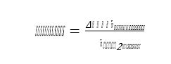
where 𝑚𝑚𝑚𝑚̇ 𝑠𝑠𝑠𝑠𝑠𝑠𝑠𝑠𝑠𝑠𝑠𝑠𝑠𝑠𝑠𝑠𝑚𝑚𝑚𝑚 is the steam flow to the reboiler heat exchanger. ∆𝐻𝐻𝐻𝐻 is the enthalpy difference between steam and condensate calculated from measured temperature and pressure, see also reboiler, steam and condensate in Figure 1. Steam pressure is typical around 2.5 barg and up to 160 °C for the tests reported in this paper.
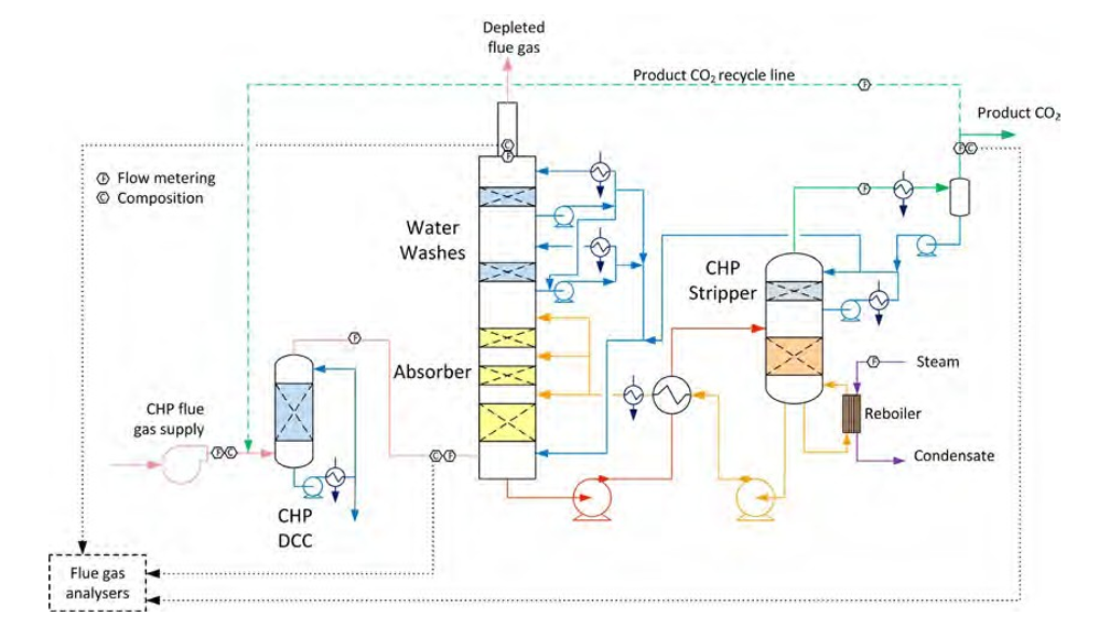
Figure 1. The TCM amine plant in CHP mode (up to 80 ton CO2 per day). Flow meters and flue gas analysers are located at absorber inlet, outlet/depleted flue gas and product flow. Captured CO2 can be recycled, see green dotted line, to increase the CO2 concentration in the flue gas flow into the absorber.
CO2 capture rate is the mass fraction of CO2 being captured out of the amount of CO2 flowing into the absorber:
Captured CO2 (𝑚𝑚𝑚𝑚̇ 𝐶𝐶𝐶𝐶𝐶𝐶𝐶𝐶2𝑐𝑐𝑐𝑐𝑠𝑠𝑠𝑠𝑐𝑐𝑐𝑐 ) in (1) and (2) can be based on CO2 in product flow (𝑚𝑚𝑚𝑚̇ 𝐶𝐶𝐶𝐶𝐶𝐶𝐶𝐶2,𝑐𝑐𝑐𝑐𝑝𝑝𝑝𝑝𝑝𝑝𝑝𝑝𝑝𝑝𝑝𝑝) leaving the stripper or on difference in mass flow of CO2 over the absorber (𝑚𝑚𝑚𝑚̇ 𝐶𝐶𝐶𝐶𝐶𝐶𝐶𝐶2𝑠𝑠𝑠𝑠𝑎𝑎𝑎𝑎𝑠𝑠𝑠𝑠,𝑖𝑖𝑖𝑖𝑖𝑖𝑖𝑖 − 𝑚𝑚𝑚𝑚̇ 𝐶𝐶𝐶𝐶𝐶𝐶𝐶𝐶2𝑠𝑠𝑠𝑠𝑎𝑎𝑎𝑎𝑠𝑠𝑠𝑠,𝑝𝑝𝑝𝑝𝑜𝑜𝑜𝑜𝑠𝑠𝑠𝑠). There are several ways of calculating CO2 capture rate [4]. In addition to this and as outlined in more details in [4,5] TCM is equipped with multiple flue gas analysers for measuring composition in and out of the absorber and out of the stripper, see Figure 1. This also includes moisture which alternatively can be calculated based on thermodynamics using temperature and pressure of the gases in question. The flow meter at the absorber outlet is unreliable and flow out of absorber is calculated from flow into the absorber assuming that all components except moisture and CO2 are conserved. The current analysis will be based on the selection of composition analysers, flow meters and calculation methods presented in Appendix B.
Lean and rich solvent loading (mole CO2 /mole amine) are calculated from laboratory analysis of liquid solvent samples that provide total inorganic carbon (mole CO2 /kg solvent) and total alkalinity (mole amine/kg solvent):
3. Optimising performance: energy
Most of the MEA-3 program was conducted with CO2 concentration at 4.2 % (wet) in the flue gas into the absorber. This was maintained by recycling captured CO2 back to the absorber inlet. This secured stable CO2 concentration in the flue gas since recycled CO2 could top the initial CO2 concentration of 3.5 to 3.9 % up to 4.2 % (wet). This CO2 level is typical for state of the art CCGT plants. Selected test series that will be discussed below are presented in Table 1.
Figure 2 shows to the left the MEA-3 test series 3 with black filled symbols and series 11 with black open symbols. These two series were operated at 47,000 Sm3/h, 24 meter absorber packing and without use of anti-foam. Compared to results from the MEA-2 campaign in 2015 [5] these two new test series resulted in a lower optimum SRD, but this may be due to several aspects and in addition the CO2 concentration in the flue gas into absorber was higher. However, during this part of the campaign the amine plant could be operated at rather high stripper bottom temperature and corresponding low lean solvent CO2 loading without the use of antifoam. Thus, the resulting optimum point was found at a higher stripper bottom temperature and lower lean CO2 loading compared to MEA-2 results, i.e. 118.1 °C /0.29 mole/mole for MEA-2 versus 121.0 °C/0.21 mole/mole for MEA-3. Results down to 3.6 GJ/ton CO2 was not achieved at 24 meter absorber packing when operated without the use of anti-foam and as will be presented below the effect anti-foam was not at all as pronounced as in the MEA-2 campaign. We acknowledge this difference in performance which could be due to several factors, however, this has not yet been concluded.
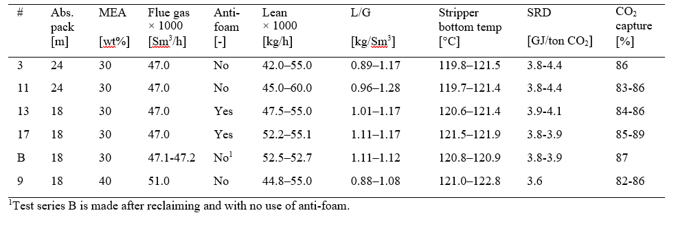
Table 1. Selected test series from MEA-3 campaign at 24 and 18 meter absorber packing, the latter operated at 30 and 40 wt% MEA. The liquid- to gas ratio (L/G) is the ratio of lean amine- to flue gas flow. SRD is based on thermal energy, see equation 1.
All SRDs and capture rates presented in Figure 2, Table 1 and Table 2 are calculated based on that captured CO2 (𝑚𝑚𝑚𝑚̇ 𝐶𝐶𝐶𝐶𝐶𝐶𝐶𝐶2𝑐𝑐𝑐𝑐𝑠𝑠𝑠𝑠𝑐𝑐𝑐𝑐 ) in equation (1) is derived from the difference in mass flow of CO2 over the absorber. Earlier reported data from MEA-2 campaign [5] was based on measured product mass flow of out of stripper. The discussion below is
based on a reassessment of these data using mass flow of CO2 over the absorber. The data points presented are made from averaging process data over a two hour time slot. This time slot also includes liquid solvent samples such that solvent CO2 loading can be calculated according to equation (3).
Performance at 18 meter absorber packing height was investigated at both 30 and 40 wt% MEA. Figure 2 shows to the right the MEA-3 test series 13 and 17 with filled and open brown symbols, respectively. The blue filled symbols are test series B without anti-foam that was executed after solvent reclaiming. The best SRDs were obtained around
3.8 GJ/ton CO2 for test series 17 which is a bit below the 24 meter tests in MEA-2 without anti-foam. The red filled symbols in Figure 2 right hand side shows MEA-3 series 9 which was operated with 51,000 Sm3/h flue gas flow, 40 wt% MEA and without the use of anti-foam. The optimum SRD is similar as the best performance from MEA-2, however, the absorber packing required was reduced from 24 meter (MEA-2) to 18 meter (MEA-3) and no use of anti- foam. Test series 9 was stopped before completion due to increasing ammonia emission and signs of corrosion i.e. increasing iron content in solvent. Thus only a limited number of parameter variations was conducted during operation at 40 wt% MEA and there might still be a potential for obtaining even lower SRDs. Another observation was that the use of anti-foam had limited effect on performance which can be seen from the brown (with anti-foam) and the blue symbols (without anti-foam) in Figure 2 to the right. Case 9-4 that was operated at 40 wt% MEA without the use of anti-foam resulted in the lowest SRD in this campaign.
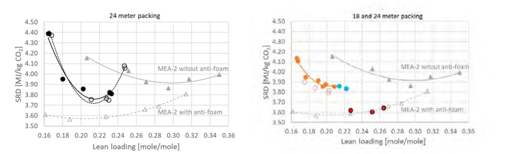
Figure 2. To the left SRD for tests utilising 24 meter absorber packing compared to results from MEA-2 in 2015 (grey symbols and lines). MEA-3 series 3 is with black filled symbols and series 11 is with black open symbols. To the right SRD for tests at 18 meter absorber packing compared to the same results from MEA-2 in 2015 (grey symbols and lines). Series 13 is with brown filled symbols, series 17 with brown open symbols, series B with blue symbols and series 9 which is with 40 wt% MEA, is with red symbols. SRDs are calculated based on difference in mass flow of CO2 over the absorber. All plots except series 9 are with 30 wt% MEA. The right and left figure present the same MEA-2 results utilising 24 meter absorber packing. Table 1 and Table 2 provide more information about the test series.
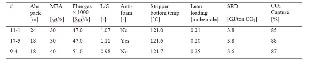
Table 2. With ref to Figure 2 operational data, SRD and capture rate for the three cases at lowest SRD values during MEA-3. SRD is based on thermal energy, see equation 1.
4. Modes of operation
Based on previous work [4,5] it was interesting to further investigate the trade-off between capital expenditure (CAPEX) and operational expenditure (OPEX) parameters for operating conditions relevant for various CCGT- and exhaust gas recycling systems with the aim of providing experimental evidence on how total capture cost can be minimized.
The flexibility of the TCM amine plant was utilized in test series with large variations in absorber packing height, flue gas flow rate, liquid- to gas flow ratio (L/G), solvent CO2 loading and inlet CO2 concentration. This experimental set-up covered a range of operating modes. Data collection and performance results such as mass balance, CO2 recovery, capture rate and SRD are according to methods described in section 2 above. Table 3 gives operational parameters and performance results for selected cases used in the cost evaluation described in section 6 below. Data from previous campaigns, MEA-1 and MEA-2 [2,4], are also included in the table for comparison.
Table 3. Test cases selected for further investigation. Case 11-1 and 9-4 are optimum modes of operation selected from Figure 2. The liquid- to gas ratio (L/G) is the ratio of lean amine- to flue gas flow. SRD is based on thermal energy, see equation 1.
The initial learning at TCM during the years 2013 and 2014 are represented by the test case MEA-1. At that time the operation was mainly with 24 meter absorber packing height and flue gas flow at 47,000 Sm3/h (80 % of design flow capacity). For capture rates between 85 to 90 % the specific reboiler duty was measured to 4.1 GJ/ton CO2.
In the MEA-2 campaign in 2015 learning from several test campaigns were implemented in the test plan. Addition of anti-foam improved especially the stripper performance. This allowed operation with full flue gas load and achievement of both high capture rates and significantly lower SRD values.
In the current MEA-3 campaign, the cases 11-1 and 5-1 are utilizing 24 meter absorber packing height and were run at 47,000 and 59,000 Sm3/h flue gas flow, respectively. The stripper performance constrained the maximum possible CO2 capture to 3,480 kg/h in the case with highest flue gas flow. The corresponding capture rate was 77%. However, during the current campaign no energy optimisation was made at 59,000 Sm3/h flue gas flow and this test was done without the use of anti-foam.
From the three cases run at 18 meter absorber packing height (cases 8-1, 9-4 and 13-2) it is seen that the benefit of 40 w% MEA is lower L/G, lower SRD and still achieving high capture rate. The low L/G and the high lean CO2 loading indicates a further potential for capturing more CO2 in this system.
The two cases run at 12 meter absorber packing height achieved rather low capture rates. The benefit of increasing the CO2 concentration in the flue gas flow into absorber from 4.2 to 5.0 % (wet) is assessed based on results from these two cases.
5. Cost assessment and cost of CO2 avoided
The economic evaluations of power and capture plants in this paper is based on standard “Cost of Electricity” (COE)- and “Cost of CO2 avoided” metrics. These calculations are based on aligned and standardized estimates and assumptions on technology process performance such as energy efficiency, CO2 generation and capture rates, see e.g. [7]. Cost estimates include CAPEX, operations and maintenance (O&M) including fuel and a set of general price and rate of return assumptions. For each case in section 6 below, a complete sized capture plant equipment list is established. Aspen In-Plant Cost Estimator (IPCE) V9 is used to estimate equipment cost. Equipment installation factors are then used to estimate total installed costs. The OPEX can be split in annual cost (of capex), power loss, maintenance, chemicals and fixed operating costs. The gas fired power plant specific cost is based on GTPro and a West Europe scenario. All calculations are furthermore carried out at:
- normalised, per unit (kWh) output from the base industrial (power) plant
- pretax, pre-financing basis
- annual cost basis, applying a capital charge factor corresponding to a standard discount factor and project time horizon
Cost of CO2 avoided ($/ton CO2 ) is calculated according to (4) below and is based on cost of electricity (COE) and CO2 emission per kWh ( CO2 emission) for a power plant with capture (cap) and without CO2 capture (no cap).
The calculated cost of CO2 avoided implicitly accounts for the capture systems’ own energy demand and its inherent CO2 emissions. The following economic assumptions are applied:
- Fuel gas price: 0.1875 US $/Sm3
- On-stream hours: 7,884 (90 %)
- Discount rate: 5 % real (pretax)
- Time horizon: 30 years
This paper will only report percentage cost reduction and no absolute cost numbers. The main reasons are that the absolute numbers are not useful for the purpose of this work and are partially confidential. In this work one consistent method and one consistent set of assumptions are used for calculating the cost, which is important for a fair comparison.
6. Cost evaluation of selected cases
The experiments targeted lowest possible absorber packing height, lowest possible L/G and SRD while maximizing the captured CO2 and capture rate. In Table 4 below the experimental data for the selected cases are scaled to a full- scale design at a fixed inlet CO2 flow of 150 ton CO2 /h and measured capture rate case by case.
In order to compare the MEA-1 and MEA-2 to MEA-3 on the same basis in the cost assessment, the CO2 inlet concentrations for these two cases are adjusted up to 4.2 % (wet) and the flue gas flow rates are reduced correspondingly, reducing the size and cost of flue gas blower, DCC and absorber. The superficial gas velocity is held constant in the DCC and absorber, reducing the diameter of these units.
The adjusted/scaled absorber packing height and the most important cost parameter, the packing volume, are calculated from the experimental data for the cases selected in the MEA-3 campaign. The scaled-up absorber volume is based on packing height utilised for each TCM test case and a scaled up cross sectional area. The latter is calculated based on TCM cross sectional area and the ratio of full-scale (150 ton CO2 /h) to TCM (case by case) CO2 inlet flow. For all scaled up cases the cross sectional areas are adjusted to fit with a superficial velocity of 2 m/s (at 0 °C, 1 atm).
Thus, packing height, see Table 4, is adjusted in order to maintain the scaled-up absorber packing volume. The packing volume per captured CO2 will be equal for each TCM and corresponding scaled up case. The data are shown in Table 4 below together with calculated lean solvent flow per kg CO2 into absorber, CO2 loading in lean and rich amine. The rich CO2 loading is calculated based on solvent flow rate and captured CO2 .
Packing volume is a major CAPEX element and for operation with 30 and 40 wt% MEA the most cost-effective packing volume demonstrated at TCM was about 37 m3/ton CO2 capture per hour for the current test conditions. This result is however, design and site specific. In case 9-4 with 40 wt% MEA the main cost reduction parameters are reduced enthalpy to reboiler (low SRD) and reduced solvent flow rate.
The case 11-1 had more packing than needed and very little CO2 is captured in the upper 6 m packed bed. The cases 11-1, 8-1 and 13-2 performed close to the MEA-2 results, while the case 5-1 was performing poorer. The flue gas flow rate was very high in this case resulting in high CO2 flow into the absorber. The rich CO2 loading was high, indicating that the solvent flow rate was too low to achieve high capture rate. Solvent flow rate was 12.02 kg solvent per kg CO2 in comparison to at least 13.50 kg solvent per kg CO2 into absorber for the best cases. In new campaigns some of the cases could be further improved if higher capture rates are obtained.
The cases 15-0 and 15-3 with 12 m absorber packing achieved the lowest packing volume per kg CO2 captured. On the other hand, the capture rate was low and the solvent flow rate was higher. This resulted in higher capture cost. These cases had in fact a too low packing volume.
In MEA-1 the packing volume was slightly higher than for the 11-1 case, solvent flow was higher and the rich loading was lower. In MEA-2 with 24 meter absorber packing height, the packing volume of 50 m3 per ton CO2 captured is on the high side compared to the MEA-3 results.
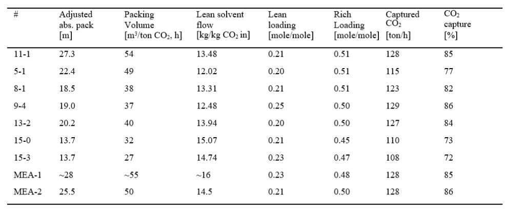
Table 4. The test cases selected for further investigation are scaled up to 150 ton of CO2/h in the flue gas into the absorber base on 2 m/s superficial velocity (at 0 °C, 1 atm) in the absorber. Case 11-1 and 9-4 are optimum cases in Figure 2 while rest of the tests documents different modes of operation.
Section 5 above introduces the economic evaluation and cost of CO2 avoided. In Figure 3 to the left the demonstrated cost reduction for the seven test cases selected from MEA-3 is presented relative to the cost of CO2 avoided of MEA-1. The demonstrated effect of increasing the CO2 concentration in flue gas into absorber from 4.2 to
5.0 % (wet) is shown by cases 15-0 and 15-3. When scaled to 150 ton CO2 /h the cost reduction for 15-0 to 15-3 is mainly due to the reduced resulting flow of flue gas, impacting the cost of the DCC, flue gas blower and absorber. Case 9-4 demonstrates the largest cost reduction contribution, i.e. 13.5 % down relative to MEA-1. This case is also presented in Figure 3 to the right (MEA-3) along with MEA-2 and a theoretically case based on 9-4 assuming 5 % CO2 (wet) in the flue gas. The latter improves the case 9-4 by about 5 % points.
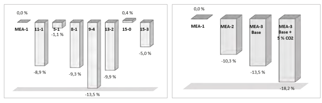
Figure 3. To the left: Demonstrated reduction in cost of CO2 avoided for seven selected MEA-3 cases. To the right: Lowering cost of CO2 avoided in campaigns MEA-1 to MEA-3. The MEA-3 is also presented with its theoretically potential if CO2 content in flue gas is 5 % (MEA-3 Base + 5
% CO2 ). Results are presented relative to assessment made for MEA-1 in 2014. Note that case 9-4 in the left plot is presented as “MEA-3 base” in the right plot.
The measures in Figure 3 do not represent radical new ways of operating or new technologies. They can rather be categorized as learning-by doing. They are typically measures relevant for the first few plants, also called FOAK – first of a kind. Since the cost reduction potential of these measures is experimentally verified in one of the world’s largest demonstration plants, the cost reduction should be highly accurate, and hence relevant for future post- combustion plants.
Based on the experience from the test campaign other reduction measures have been studies on a theoretical basis in order to investigate future potential for reducing cost of CO2 avoided. A theoretical parameter study has been made based on case 9-4, referred as “MEA-3 Base” in Figure 4. The following elements have been assessed:
- Reduce from 2 × 3 meter wash section to 1 × 3 meter wash section
- Reduce solvent consumption from 1.6 kg/ton CO2 down to 0.3 kg/ton CO2 [8,9]
- Increase CO2 capture rate from 86 to 90 %
- Reduce steam consumption to achieve SRD of 3.1 GJ/ton CO2 (other solvents than MEA)
- Increasing CO2 content in flue gas from 4.2 up to 5 %
These measures are considered to be realistic. Most of the numbers are reported in the post-combustion literature and seem reasonable. In addition to these measures reduced manning is also included in the parameter study for illustration:
- Reduced manning from 4 operators per shift to 1 operator per shift
Figure 4 shows the cumulative effect for cost of CO2 avoided from these 6 elements. Solvent and process development relates to the first five items. The assumptions on operators before and after reduction is not based on TCM experience. The second last element corresponds to state of the art CCGT plants that are expected to be operated at 5 % CO2 . The five first elements improves the “MEA-3 Base” by 17.1 % while utilizing all six elements results in 21.5 % improvement.
All in all, these initiatives will represent a reduction in cost of CO2 avoided of the order of 30 % when compared to MEA-1. However, note that these measures are not necessary cumulative, i.e. all combinations may not be possible at the same time.
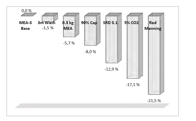
Figure 4. Relative cost of CO2 avoided based test case 9-4 (MEA-3 Base) and a theoretical parameter study involving 6 cost reduction initiatives introduced on top of each other.
7. Conclusion
Different modes of operation with cost saving potential were executed as part of the MEA-3 campaign at TCM from December 2017 to February 2018. The target was to explore learning from five years of operation at TCM with respect to overall cost reduction potential using the relative cost of CO2 avoided metric. The new results were therefore compared to those reported from the MEA-1 and MEA-2 campaigns. The investigation of optimum energy performance identified that SRD values below 3.6 GJ/ton CO2 for MEA are challenging to achieve with 30 wt% MEA and a CCGT like flue gas. This performance is achieved at TCM with a conventional amine plant and may be optimized with an advance process plant. In the cost reduction part of the investigation the level of 10 % cost reduction in cost of CO2 avoided as achieved in MEA-2 was confirmed with the new experiments. Packing volume is a major CAPEX element and the most cost-effective packing volume demonstrated based on TCM equipment, was about 37 m3/ton CO2 capture per hour for the current test conditions. The lowest cost of CO2 avoided was demonstrated when using MEA at 40 wt% and 18 meter absorber packing height. Compared with MEA-1 results a cost reduction of 13.5% was demonstrated. There is likely a further cost reduction potential of 5 %-points for this case. This is based on results from tests when the flue gas CO2 concentration was increased from 4.2 to 5.0 % (wet). Finally, a theoretical parameter variation showed a potential cost reduction of around 20 % compared with MEA-3 Base. Compared to MEA-1 this amounts to a reduction potential of the order of 30 %. However, all combinations may not be possible at the same time.
It is important to notice that these results are generated at one of the world’s largest capture demonstration units, and that it is the first time that such a structured campaign is executed. Similar testing can be carried out with different amine-based solvents. Therefore, these results at TCM scale represent a very relevant basis for scale up and industrial design of amine solvent capture technologies.
Acknowledgements
The authors gratefully acknowledge the staff of TCM DA, Gassnova, Equinor, Shell and Total for their contribution and work at the TCM DA facility. The authors also gratefully acknowledge Gassnova, Equinor, Shell, and Total as the owners of TCM DA for their financial support and contributions.
Appendix A
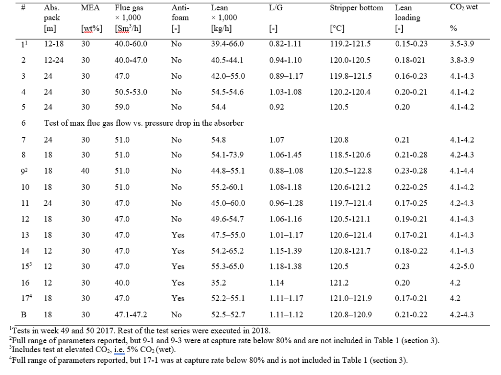
Table A1. The test series during MEA-3, 2017-2018.
Appendix B
Table B1. Selected instruments and calculation methods for analysing test data.
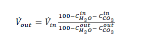
With ref to Table B1 the volume flow out of the absorber (𝑉out) is calculated from volume flow into (Vin) the
absorber assuming all components except water (𝐶H2O) and CO2 (𝐶CO2) are conserved:
References
- The Open-source Centre at TCM, https://catchingourfuture.com/
- Hamborg ES, Smith V, Cents T, Brigman N, Falk-Pedersen O, de Cazenove T, Chhaganl M, Feste JK, Ullestad Ø, Ulvatn H, Gorset O, Askestad I, Gram LK, Fostås BF, Shah MI, Maxson A, Thimsen D. Results from MEA testing at the CO2 Technology Centre Mongstad. Part II: Verification of baseline results. Energy Procedia, Volume 63, 2014, p. 5994-6011.
- Thimsen D, Maxson A, Smith V, Cents T, Falk-Pedersen O, Gorset O, Hamborg ES. Results from MEA testing at the CO2 Technology Centre Mongstad. Part I: Post-Combustion CO2 capture testing methodology. Energy Procedia, Volume 63, 2014, p. 5938-5958.
- Faramarzi L, Thimsen D, Hume S, Maxon A, Watson G, Pedersen S, Gjernes E, Fostås BF, Lombardo G, Cents T, Morken AK, Shah MI, de Cazenove T, Hamborg ES, Results from MEA Testing at the CO2 Technology Centre Mongstad: Verification of Baseline Results in 2015. Energy Procedia, Volume 114, 2017, p 1128-1145.
- Gjernes E, Pedersen S, Cents T, Watson G, Fostås BF, Shah MI, Lombardo G, Desvignes C, Flø NE, Morken AK, de Cazenove T, Faramarzi L, Hamborg ES. Results from 30 wt% MEA performance testing at the CO2 Technology Centre Mongstad. Energy Procedia, Volume 114, 2017, p 1146-1157.
- Flø NE, Faramarzi L, Iversen F, Kleppe ER, Graver B, Byntesen HN, Johnsen K. Assessment of material selection for the CO2 absorption process with aqueous MEA solution based on results from corrosion monitoring at Technology Centre Mongstad. To be presented at GHGT- 14, 2018, Melbourne, Australia.
- Cost and Performance Baseline for Fossil Energy Plants Volume 1a: Bituminous Coal (PC) and Natural Gas to Electricity Revision 3, July 6, 2015, DOE/NETL-2015/1723.
- Morken, AK, Pedersen S, Kleppe ER, Wisthaler A,Vernstad K, Ullestad Ø, Flø NE, Faramarzi L, Hamborg ES. Degradation and Emission Results of Amine Plant Operations from MEA Testing at the CO2 Technology Centre Mongstad. Energy Procedia, Volume 114, 2017, p 1245- 1262.
- Gorset O, Knudsen JN, Bade OM, Askestad I. Results from Testing of Aker Solutions Advanced Amine Solvents at CO2 Technology Centre Mongstad. Energy Procedia, Volume 63, 2014, p 6267-6280.